Seurat - Comparison between single cell and nuclei RNA-seq for 3 datasets
Matthieu Sieber
Compiled: May 28, 2025
Disclaimer on the Use of Artificial Intelligence
Parts of this analysis and associated code were developed with the assistance of artificial intelligence tools, including ChatGPT (OpenAI). These tools were used to help clarify R programming syntax, improve code readability, and troubleshoot technical issues. All final decisions regarding code structure, data interpretation, and scientific content were made by the author.
Introduction
This document presents the integration of three single-cell and single-nucleus RNA sequencing (sc/snRNA-seq) datasets derived from Aedes aegypti midgut samples. The aim of this analysis is to harmonize these datasets into a common embedding, in order to allow robust identification and comparison of cell populations across different experimental conditions and technologies.
Prior to integration, each dataset underwent quality control, normalization, and dimensionality reduction using Seurat. The datasets were then merged and integrated using [integration method, e.g., Seurat’s CCA or Harmony], followed by clustering and visualization with UMAP. This approach enables the assessment of shared and specific cell populations and the identification of potential batch effects between single-cell and single-nucleus data.
All steps described here were performed using R (version X.X.X) and Seurat (version X.X.X), and the analysis is fully reproducible. The analysis is based on the vignettes from Satijalab https://satijalab.org/seurat/ and especially the tutorial for Seurat analysis with pbmc dataset https://satijalab.org/seurat/articles/integration_introduction and the integration with Seurat v5 https://satijalab.org/seurat/articles/seurat5_integration.
Datasets:
Gene expression level in Aedes aegypti midgut four days post blood fed (single cell), https://www.ncbi.nlm.nih.gov/geo/query/acc.cgi?acc=GSM8282824
A cell atlas of the adult female Aedes aegypti midgut revealed by single-cell RNA sequencing, replicate 1, https://www.ncbi.nlm.nih.gov/geo/query/acc.cgi?acc=GSM7872696
A single-nucleus transcriptomic atlas of the adult Aedes aegypti mosquito, https://cells.ucsc.edu/mosquito/t012/t012.h5ad
Setup R
Setup the Seurat Objects
We start by reading in the data. The Read10X() function
reads in the output of the cellranger
pipeline from 10X, returning a unique molecular identified (UMI) count
matrix. The values in this matrix represent the number of molecules for
each feature (i.e. gene; row) that are detected in each cell
(column).
We next use the count matrix to create a Seurat object.
The object serves as a container that contains both data (like the count
matrix) and analysis (like PCA, or clustering results) for a single-cell
dataset. For a technical discussion of the Seurat object
structure, check out our GitHub Wiki. For
example, the count matrix is stored in
pbmc[["RNA"]]@counts.
Finally we merge the two datasets into one object for downstream analyses (example from https://satijalab.org/seurat/articles/seurat5_merge_vignette)
library(Matrix)
library(SeuratObject)
library(dplyr)
library(Seurat)
library(patchwork)
library(clustree)
library(reticulate)
use_python("/usr/local/bin/python3", required = TRUE)
library(sceasy)
library(scCustomize)
library(anndata)
library(ggplot2)
library(openxlsx) # for excel tables
library(tidyr)
library(writexl)

# Set the working directory
setwd("~/R/backups/cellvsnuclei")
message("Working directory set to: ", getwd())

# Load the 2 datasets for single cell
midcont.data <- Read10X(data.dir = '~/R/data/zika/control')
midcell1.data <- Read10X(data.dir = "~/R/data/cell/rep1")

# Backup the rawdata for single nuclei
anndata <- import("anndata", convert = FALSE)
midnucatlas.data <- anndata$read_h5ad(path.expand("~/R/data/atlas/t012.h5ad"))

midnucatlas.raw.py <- midnucatlas.data$layers$get("raw_data")
midnucatlas.raw <- py_to_r(midnucatlas.raw.py)

## Convert to dgCMatrix if not
if (!inherits(midnucatlas.raw, "dgCMatrix")) {
  midnucatlas.raw <- as(midnucatlas.raw, "dgCMatrix")
}

## Invert the matrix because features and events inverted
midnucatlas.raw <- t(midnucatlas.raw)
rownames(midnucatlas.raw) <- py_to_r(midnucatlas.data$var_names)   # features
colnames(midnucatlas.raw) <- py_to_r(midnucatlas.data$obs_names)   # events

# Initialize the Seurat objects with the raw (non-normalized data)
midcont <- CreateSeuratObject(counts = midcont.data, project = "midgut_zika_control", min.cells = 3, min.features = 100)
midcell1 <- CreateSeuratObject(counts = midcell1.data, project = "midgut_cell_rep1", min.cells = 3, min.features = 100)
midnucatlas <- CreateSeuratObject(counts = midnucatlas.raw, project = "midgut_nuclei_atlas", min.cells = 3, min.features = 100)

# Merge all Seurat objects for further analysis
midgut <- merge(midcont, y = c(midcell1, midnucatlas), add.cell.ids = c("control", "cell1", "nuclei_atlas"), project = "midgut_integration")

# Show the number of events by origine
table(midgut$orig.ident)
##
## midgut_cell_rep1 midgut_nuclei_atlas midgut_zika_control
## 11870 18094 5469Check if nonnormalized data
This chunk is necessary to verify that the data we use are the raw data or they are already normalized and scaled.
names(midgut[["RNA"]]@layers)## [1] "counts.midgut_zika_control" "counts.midgut_cell_rep1"
## [3] "counts.midgut_nuclei_atlas"layer1 <- midgut[["RNA"]]@layers[["counts.midgut_zika_control"]]
layer2 <- midgut[["RNA"]]@layers[["counts.midgut_cell_rep1"]]
layer3 <- midgut[["RNA"]]@layers[["counts.midgut_nuclei_atlas"]]
summary(as.numeric(layer1))## Min. 1st Qu. Median Mean 3rd Qu. Max.
## 0.0000 0.0000 0.0000 0.1181 0.0000 3611.0000summary(as.numeric(layer2))## Min. 1st Qu. Median Mean 3rd Qu. Max.
## 0.000e+00 0.000e+00 0.000e+00 4.160e-01 0.000e+00 1.151e+05summary(as.numeric(layer3))## Min. 1st Qu. Median Mean 3rd Qu. Max.
## 0.000e+00 0.000e+00 0.000e+00 7.417e-01 0.000e+00 2.636e+04all(layer1 == round(layer1)) # to be TRUE ## [1] TRUEall(layer1 >= 0) # to be TRUE## [1] TRUEall(layer2 == round(layer2)) # to be TRUE## [1] TRUEall(layer2 >= 0) # to be TRUE## [1] TRUEall(layer3 == round(layer3)) # to be TRUE## [1] TRUEall(layer3 >= 0) # to be TRUE## [1] TRUEAdd technique condition
This code add a new column in the data to set the 2 first datasets as single cell and the last one as nuclei.
midgut$technique <- ifelse(
  midgut$orig.ident %in% ("midgut_nuclei_atlas"),
  "nuclei",
  "cell"
)

# Show the number of cells for each technique
table(midgut$technique)
##
## cell nuclei
## 17339 18094Standard pre-processing workflow
The steps below encompass the standard pre-processing workflow for scRNA-seq data in Seurat. These represent the selection and filtration of cells based on QC metrics, data normalization and scaling, and the detection of highly variable features.
QC and selecting cells for further analysis
Seurat allows you to easily explore QC metrics and filter cells based on any user-defined criteria. A few QC metrics commonly used by the community include
- The number of unique genes detected in each cell.
- Low-quality cells or empty droplets will often have very few genes
- Cell doublets or multiplets may exhibit an aberrantly high gene count
- Similarly, the total number of molecules detected within a cell (correlates strongly with unique genes)
- The percentage of reads that map to the mitochondrial genome
- Low-quality / dying cells often exhibit extensive mitochondrial contamination
- We calculate mitochondrial QC metrics with the
PercentageFeatureSet()function, which calculates the percentage of counts originating from a set of features - We use the set of all genes starting with
MT-as a set of mitochondrial genes
# The [[ operator can add columns to object metadata. This is a great place to stash QC stats
midgut[["percent.mt"]] <- PercentageFeatureSet(midgut, pattern = "AAEL018658|AAEL018662|AAEL018664|AAEL018667|AAEL018668|AAEL018669|AAEL018671|AAEL018678|AAEL018680|AAEL018681|AAEL018684|AAEL018685|AAEL018687")
In the example below, we visualize QC metrics, and use these to filter cells.
- We filter cells that have unique feature counts over 6,500 or less than 100
- We filter cells that have >30% mitochondrial counts, according to the analyze made by Wang et al.
#Visualize QC metrics as a violin plot
VlnPlot(midgut, features = c("nFeature_RNA", "nCount_RNA", "percent.mt"), ncol = 3)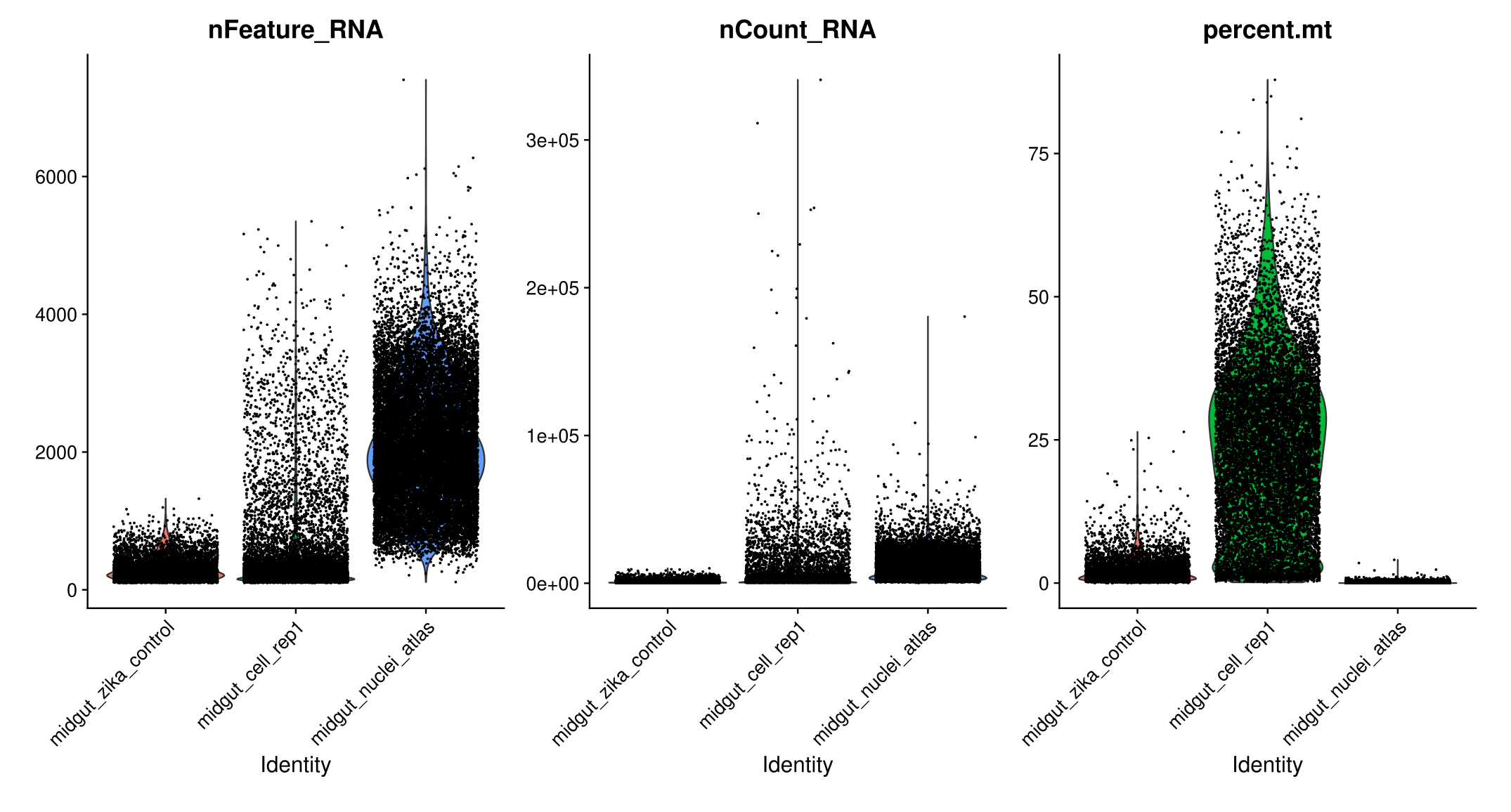
# FeatureScatter is typically used to visualize feature-feature relationships, but can be used for anything calculated by the object, i.e. columns in object metadata, PC scores etc.

plot1 <- FeatureScatter(midgut, feature1 = "nCount_RNA", feature2 = "percent.mt")
plot2 <- FeatureScatter(midgut, feature1 = "nCount_RNA", feature2 = "nFeature_RNA")
plot1 + plot2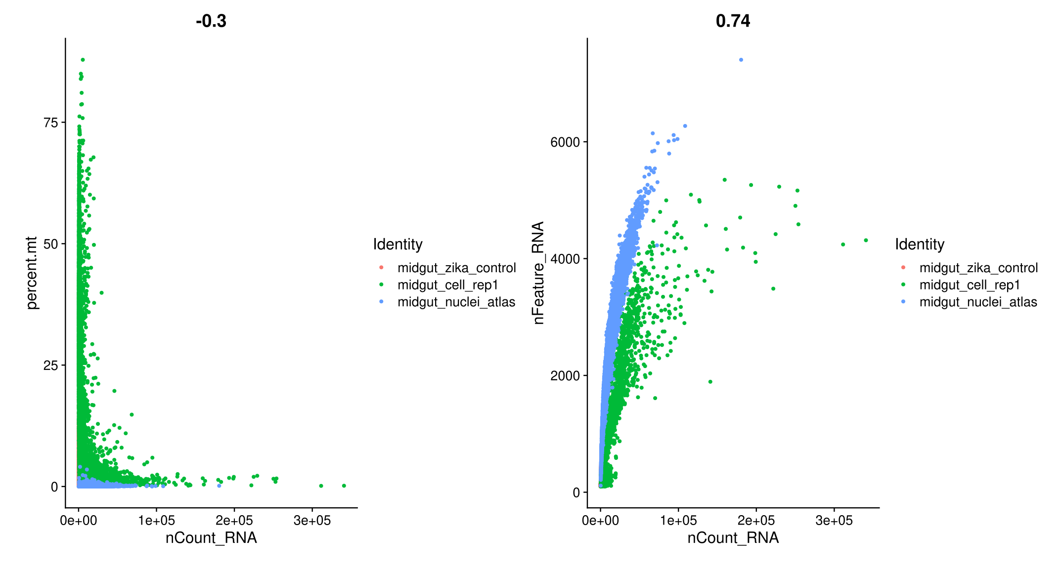
# Chen and Wang used min of 100 genes, Wang used 30% mitochondrial and 6500 max genes
midgut <- subset(midgut, subset = nFeature_RNA >= 100 & nFeature_RNA < 6500 & percent.mt < 30)

# Visualize QC metrics as ridge plots
RidgePlot(midgut, features = c("nFeature_RNA", "nCount_RNA", "percent.mt"), ncol = 1)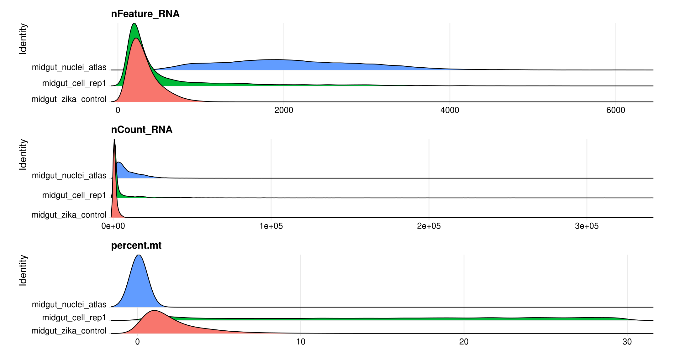
# How many cells remain after filtering
table(midgut$orig.ident)
##
## midgut_cell_rep1 midgut_nuclei_atlas midgut_zika_control
## 7850 18093 5467Normalizing the data
After removing unwanted cells from the dataset, the next step is to
normalize the data. By default, we employ a global-scaling normalization
method “LogNormalize” that normalizes the feature expression
measurements for each cell by the total expression, multiplies this by a
scale factor (10,000 by default), and log-transforms the result.
Normalized values are stored in midgut[["RNA"]]@data.
midgut <- NormalizeData(midgut)Identification of highly variable features (feature selection)
We next calculate a subset of features that exhibit high cell-to-cell variation in the dataset (i.e, they are highly expressed in some cells, and lowly expressed in others). We and others have found that focusing on these genes in downstream analysis helps to highlight biological signal in single-cell datasets.
Our procedure in Seurat is described in detail here, and improves
on previous versions by directly modeling the mean-variance relationship
inherent in single-cell data, and is implemented in the
FindVariableFeatures() function. By default, we return
2,000 features per dataset. These will be used in downstream analysis,
like PCA.
midgut <- FindVariableFeatures(midgut, selection.method = 'vst', nfeatures = 2000)

# Identify the 10 most highly variable genes
top10 <- head(VariableFeatures(midgut), 10)

# plot variable features with and without labels
plot1 <- VariableFeaturePlot(midgut)
plot2 <- LabelPoints(plot = plot1, points = top10, repel = TRUE)
plot1 + plot2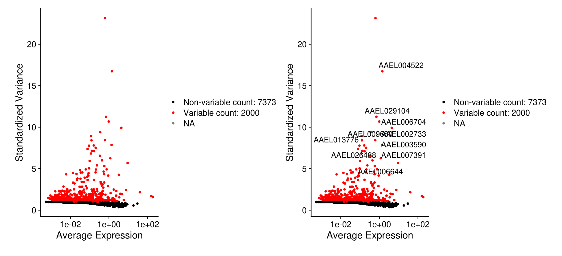
Scaling the data
Next, we apply a linear transformation (‘scaling’) that is a standard
pre-processing step prior to dimensional reduction techniques like PCA.
The ScaleData() function:
- Shifts the expression of each gene, so that the mean expression across cells is 0
- Scales the expression of each gene, so that the variance across cells is 1
- This step gives equal weight in downstream analyses, so that highly-expressed genes do not dominate
- The results of this are stored in
midgut[["RNA"]]@scale.data
all.genes <- rownames(midgut)
midgut <- ScaleData(midgut, features = all.genes)
Perform linear dimensional reduction
Next we perform PCA on the scaled data. By default, only the
previously determined variable features are used as input, but can be
defined using features argument if you wish to choose a
different subset.
midgut <- RunPCA(midgut, features = VariableFeatures(object = midgut))Seurat provides several useful ways of visualizing both cells and
features that define the PCA, including VizDimReduction(),
DimPlot(), and DimHeatmap()
# Examine and visualize PCA results a few different ways
print(midgut[['pca']], dims = 1:5, nfeatures = 5)
## PC_ 1
## Positive: AAEL007818, AAEL001703, AAEL001863, AAEL017022, AAEL013623
## Negative: AAEL023512, AAEL019563, AAEL011359, AAEL019671, AAEL004572
## PC_ 2
## Positive: AAEL004798, AAEL004930, AAEL000428, AAEL014516, AAEL022995
## Negative: AAEL021073, AAEL010783, AAEL013600, AAEL018334, AAEL004396
## PC_ 3
## Positive: AAEL014246, AAEL018334, AAEL001061, AAEL010382, AAEL003139
## Negative: AAEL005895, AAEL002769, AAEL005692, AAEL018324, AAEL018153
## PC_ 4
## Positive: AAEL018334, AAEL003139, AAEL001168, AAEL009024, AAEL005464
## Negative: AAEL012091, AAEL022387, AAEL026555, AAEL009837, AAEL019835
## PC_ 5
## Positive: AAEL006011, AAEL014246, AAEL002309, AAEL009680, AAEL013885
## Negative: AAEL020061, AAEL028205, AAEL000549, AAEL009473, AAEL019974VizDimLoadings(midgut, dims = 1:2, reduction = 'pca')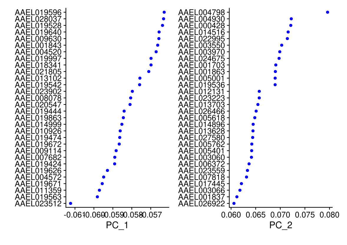
DimPlot(midgut, reduction = 'pca')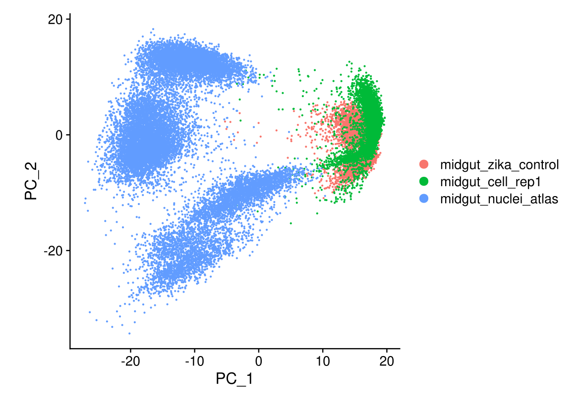
In particular DimHeatmap() allows for easy exploration
of the primary sources of heterogeneity in a dataset, and can be useful
when trying to decide which PCs to include for further downstream
analyses. Both cells and features are ordered according to their PCA
scores. Setting cells to a number plots the ‘extreme’ cells
on both ends of the spectrum, which dramatically speeds plotting for
large datasets. Though clearly a supervised analysis, we find this to be
a valuable tool for exploring correlated feature sets.
DimHeatmap(midgut, dims = 1, cells = 500, balanced = TRUE)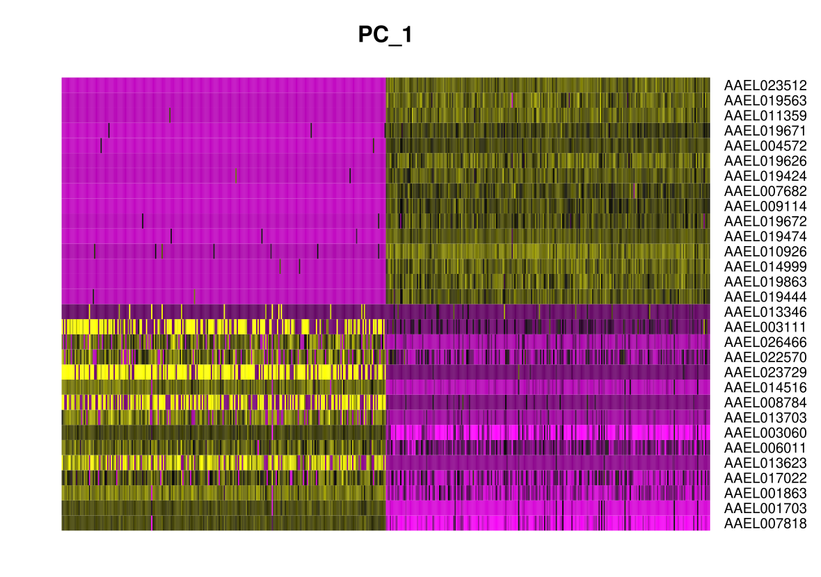
DimHeatmap(midgut, dims = 1:21, cells = 500, balanced = TRUE)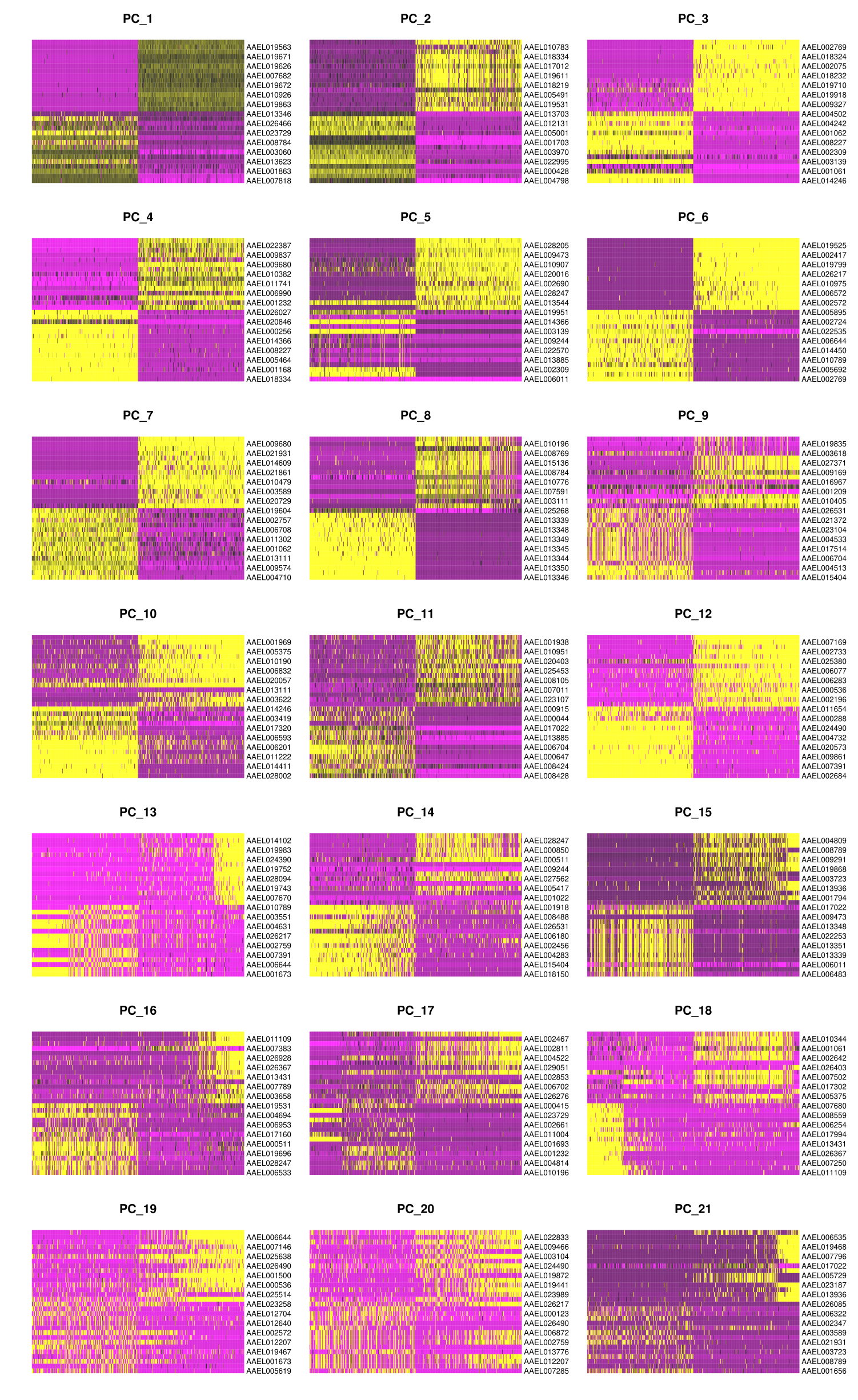
Determine the ‘dimensionality’ of the dataset
To overcome the extensive technical noise in any single feature for scRNA-seq data, Seurat clusters cells based on their PCA scores, with each PC essentially representing a ‘metafeature’ that combines information across a correlated feature set. The top principal components therefore represent a robust compression of the dataset. However, how many components should we choose to include? 10? 20? 100?
In Macosko et al, we implemented a resampling test inspired by the JackStraw procedure. We randomly permute a subset of the data (1% by default) and rerun PCA, constructing a ‘null distribution’ of feature scores, and repeat this procedure. We identify ‘significant’ PCs as those who have a strong enrichment of low p-value features.
# NOTE: This process can take a long time for big datasets, comment out for expediency. More approximate techniques such as those implemented in ElbowPlot() can be used to reduce computation time
#midgut <- JackStraw(midgut, num.replicate = 100)
#midgut <- ScoreJackStraw(midgut, dims = 1:20)
The JackStrawPlot() function provides a visualization
tool for comparing the distribution of p-values for each PC with a
uniform distribution (dashed line). ‘Significant’ PCs will show a strong
enrichment of features with low p-values (solid curve above the dashed
line). In this case it appears that there is a sharp drop-off in
significance after the first 10-12 PCs.
#JackStrawPlot(midgut, dims = 1:20)An alternative heuristic method generates an ‘Elbow plot’: a ranking
of principle components based on the percentage of variance explained by
each one (ElbowPlot() function). In this example, we can
observe an ‘elbow’ around PC9-10, suggesting that the majority of true
signal is captured in the first 10 PCs.
ElbowPlot(midgut)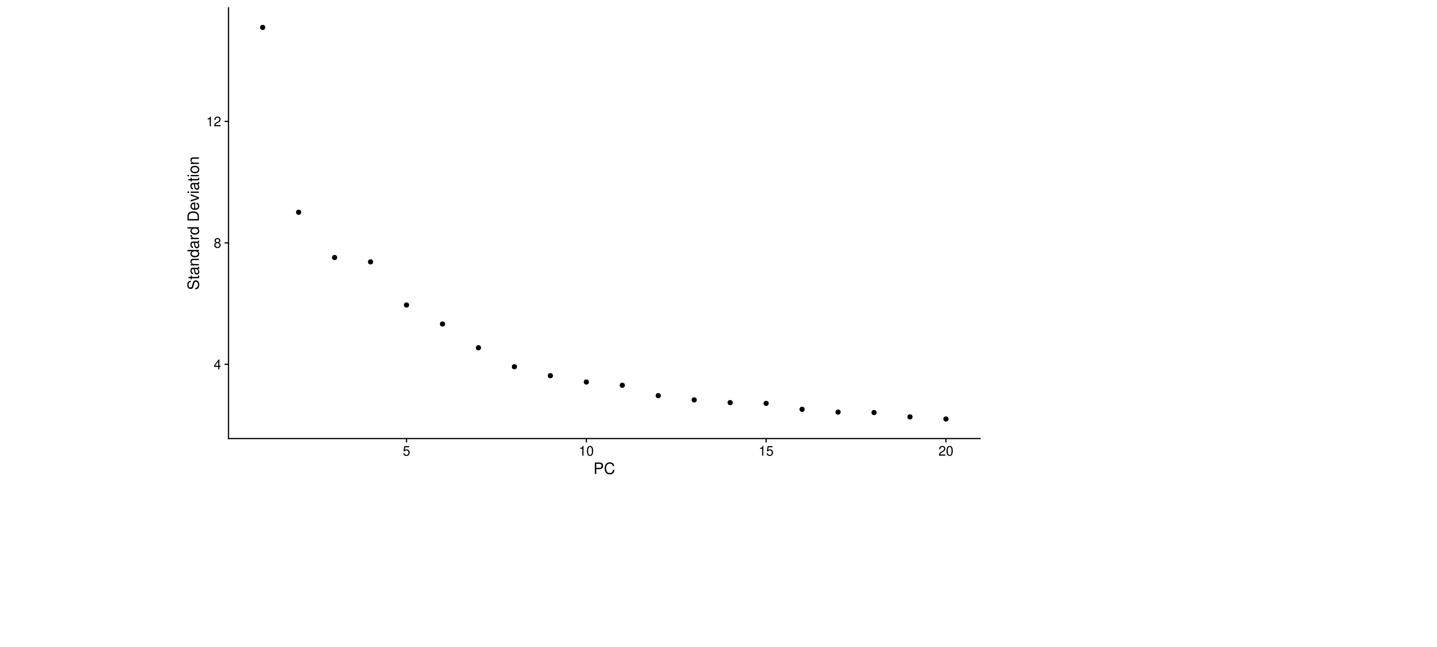
Identifying the true dimensionality of a dataset – can be challenging/uncertain for the user. We therefore suggest these three approaches to consider. The first is more supervised, exploring PCs to determine relevant sources of heterogeneity, and could be used in conjunction with GSEA for example. The second implements a statistical test based on a random null model, but is time-consuming for large datasets, and may not return a clear PC cutoff. The third is a heuristic that is commonly used, and can be calculated instantly. In this example, all three approaches yielded similar results, but we might have been justified in choosing anything between PC 7-12 as a cutoff.
We chose 10 (15) here, but encourage users to consider the following:
- Dendritic cell and NK aficionados may recognize that genes strongly associated with PCs 12 and 13 define rare immune subsets (i.e. MZB1 is a marker for plasmacytoid DCs). However, these groups are so rare, they are difficult to distinguish from background noise for a dataset of this size without prior knowledge.
- We encourage users to repeat downstream analyses with a different number of PCs (10, 15, or even 50!). As you will observe, the results often do not differ dramatically.
- We advise users to err on the higher side when choosing this parameter. For example, performing downstream analyses with only 5 PCs does significantly and adversely affect results.
Cluster the cells
Seurat v3 applies a graph-based clustering approach, building upon initial strategies in (Macosko et al). Importantly, the distance metric which drives the clustering analysis (based on previously identified PCs) remains the same. However, our approach to partitioning the cellular distance matrix into clusters has dramatically improved. Our approach was heavily inspired by recent manuscripts which applied graph-based clustering approaches to scRNA-seq data [SNN-Cliq, Xu and Su, Bioinformatics, 2015] and CyTOF data [PhenoGraph, Levine et al., Cell, 2015]. Briefly, these methods embed cells in a graph structure - for example a K-nearest neighbor (KNN) graph, with edges drawn between cells with similar feature expression patterns, and then attempt to partition this graph into highly interconnected ‘quasi-cliques’ or ‘communities’.
As in PhenoGraph, we first construct a KNN graph based on the
euclidean distance in PCA space, and refine the edge weights between any
two cells based on the shared overlap in their local neighborhoods
(Jaccard similarity). This step is performed using the
FindNeighbors() function, and takes as input the previously
defined dimensionality of the dataset (first 10 PCs).
To cluster the cells, we next apply modularity optimization
techniques such as the Louvain algorithm (default) or SLM [SLM, Blondel
et al., Journal of Statistical Mechanics], to iteratively
group cells together, with the goal of optimizing the standard
modularity function. The FindClusters() function implements
this procedure, and contains a resolution parameter that sets the
‘granularity’ of the downstream clustering, with increased values
leading to a greater number of clusters. We find that setting this
parameter between 0.4-1.2 typically returns good results for single-cell
datasets of around 3K cells. Optimal resolution often increases for
larger datasets. The clusters can be found using the
Idents() function.
Clustree is used to determine the good choice of resolution by indacting the poplations for each resolution with a plot tree. Before running this clustree, we first have to run a high resolution clustering to base the clustree.
midgut <- FindNeighbors(midgut, dims = 1:15)
midgut <- FindClusters(midgut, resolution = 2)
## Modularity Optimizer version 1.3.0 by Ludo Waltman and Nees Jan van Eck
##
## Number of nodes: 31410
## Number of edges: 1084470
##
## Running Louvain algorithm...
## Maximum modularity in 10 random starts: 0.8727
## Number of communities: 45
## Elapsed time: 4 seconds# Look at cluster IDs of the first 10 cells
head(Idents(midgut), 10)## control_AAACCTGAGTGGTAAT-1 control_AAACCTGAGTTGCAGG-1
## 13 26
## control_AAACCTGCAATCGGTT-1 control_AAACCTGCACATTCGA-1
## 5 26
## control_AAACCTGCAGCTCGCA-1 control_AAACCTGCATCGACGC-1
## 13 4
## control_AAACCTGGTGTTCTTT-1 control_AAACCTGTCAGCCTAA-1
## 13 13
## control_AAACCTGTCAGTGTTG-1 control_AAACCTGTCCCTAATT-1
## 4 4
## 45 Levels: 0 1 2 3 4 5 6 7 8 9 10 11 12 13 14 15 16 17 18 19 20 21 22 23 ... 44# cluster assignments at multiple resolutions
resolutions <- c(0.1, 0.2, 0.3, 0.4, 0.5, 0.6, 0.7, 0.8, 0.9, 1.0, 1.1, 1.2, 1.3, 1.4, 1.5, 1.6, 1.7, 1.8, 1.9, 2.0) # Example resolutions
for (res in resolutions) {
name <- paste0("RNA_snn_res.", res)
midgut <- FindClusters(midgut, resolution = res, name = name)
}## Modularity Optimizer version 1.3.0 by Ludo Waltman and Nees Jan van Eck
##
## Number of nodes: 31410
## Number of edges: 1084470
##
## Running Louvain algorithm...
## Maximum modularity in 10 random starts: 0.9794
## Number of communities: 13
## Elapsed time: 4 seconds## Modularity Optimizer version 1.3.0 by Ludo Waltman and Nees Jan van Eck
##
## Number of nodes: 31410
## Number of edges: 1084470
##
## Running Louvain algorithm...
## Maximum modularity in 10 random starts: 0.9670
## Number of communities: 19
## Elapsed time: 5 seconds## Modularity Optimizer version 1.3.0 by Ludo Waltman and Nees Jan van Eck
##
## Number of nodes: 31410
## Number of edges: 1084470
##
## Running Louvain algorithm...
## Maximum modularity in 10 random starts: 0.9576
## Number of communities: 20
## Elapsed time: 4 seconds## Modularity Optimizer version 1.3.0 by Ludo Waltman and Nees Jan van Eck
##
## Number of nodes: 31410
## Number of edges: 1084470
##
## Running Louvain algorithm...
## Maximum modularity in 10 random starts: 0.9491
## Number of communities: 21
## Elapsed time: 5 seconds## Modularity Optimizer version 1.3.0 by Ludo Waltman and Nees Jan van Eck
##
## Number of nodes: 31410
## Number of edges: 1084470
##
## Running Louvain algorithm...
## Maximum modularity in 10 random starts: 0.9412
## Number of communities: 25
## Elapsed time: 4 seconds## Modularity Optimizer version 1.3.0 by Ludo Waltman and Nees Jan van Eck
##
## Number of nodes: 31410
## Number of edges: 1084470
##
## Running Louvain algorithm...
## Maximum modularity in 10 random starts: 0.9340
## Number of communities: 28
## Elapsed time: 5 seconds## Modularity Optimizer version 1.3.0 by Ludo Waltman and Nees Jan van Eck
##
## Number of nodes: 31410
## Number of edges: 1084470
##
## Running Louvain algorithm...
## Maximum modularity in 10 random starts: 0.9281
## Number of communities: 32
## Elapsed time: 4 seconds## Modularity Optimizer version 1.3.0 by Ludo Waltman and Nees Jan van Eck
##
## Number of nodes: 31410
## Number of edges: 1084470
##
## Running Louvain algorithm...
## Maximum modularity in 10 random starts: 0.9231
## Number of communities: 32
## Elapsed time: 4 seconds## Modularity Optimizer version 1.3.0 by Ludo Waltman and Nees Jan van Eck
##
## Number of nodes: 31410
## Number of edges: 1084470
##
## Running Louvain algorithm...
## Maximum modularity in 10 random starts: 0.9178
## Number of communities: 33
## Elapsed time: 4 seconds## Modularity Optimizer version 1.3.0 by Ludo Waltman and Nees Jan van Eck
##
## Number of nodes: 31410
## Number of edges: 1084470
##
## Running Louvain algorithm...
## Maximum modularity in 10 random starts: 0.9123
## Number of communities: 33
## Elapsed time: 4 seconds## Modularity Optimizer version 1.3.0 by Ludo Waltman and Nees Jan van Eck
##
## Number of nodes: 31410
## Number of edges: 1084470
##
## Running Louvain algorithm...
## Maximum modularity in 10 random starts: 0.9074
## Number of communities: 36
## Elapsed time: 4 seconds## Modularity Optimizer version 1.3.0 by Ludo Waltman and Nees Jan van Eck
##
## Number of nodes: 31410
## Number of edges: 1084470
##
## Running Louvain algorithm...
## Maximum modularity in 10 random starts: 0.9028
## Number of communities: 39
## Elapsed time: 4 seconds## Modularity Optimizer version 1.3.0 by Ludo Waltman and Nees Jan van Eck
##
## Number of nodes: 31410
## Number of edges: 1084470
##
## Running Louvain algorithm...
## Maximum modularity in 10 random starts: 0.8996
## Number of communities: 38
## Elapsed time: 4 seconds## Modularity Optimizer version 1.3.0 by Ludo Waltman and Nees Jan van Eck
##
## Number of nodes: 31410
## Number of edges: 1084470
##
## Running Louvain algorithm...
## Maximum modularity in 10 random starts: 0.8942
## Number of communities: 39
## Elapsed time: 4 seconds## Modularity Optimizer version 1.3.0 by Ludo Waltman and Nees Jan van Eck
##
## Number of nodes: 31410
## Number of edges: 1084470
##
## Running Louvain algorithm...
## Maximum modularity in 10 random starts: 0.8906
## Number of communities: 39
## Elapsed time: 4 seconds## Modularity Optimizer version 1.3.0 by Ludo Waltman and Nees Jan van Eck
##
## Number of nodes: 31410
## Number of edges: 1084470
##
## Running Louvain algorithm...
## Maximum modularity in 10 random starts: 0.8873
## Number of communities: 40
## Elapsed time: 4 seconds## Modularity Optimizer version 1.3.0 by Ludo Waltman and Nees Jan van Eck
##
## Number of nodes: 31410
## Number of edges: 1084470
##
## Running Louvain algorithm...
## Maximum modularity in 10 random starts: 0.8836
## Number of communities: 41
## Elapsed time: 5 seconds## Modularity Optimizer version 1.3.0 by Ludo Waltman and Nees Jan van Eck
##
## Number of nodes: 31410
## Number of edges: 1084470
##
## Running Louvain algorithm...
## Maximum modularity in 10 random starts: 0.8798
## Number of communities: 41
## Elapsed time: 4 seconds## Modularity Optimizer version 1.3.0 by Ludo Waltman and Nees Jan van Eck
##
## Number of nodes: 31410
## Number of edges: 1084470
##
## Running Louvain algorithm...
## Maximum modularity in 10 random starts: 0.8764
## Number of communities: 43
## Elapsed time: 4 seconds## Modularity Optimizer version 1.3.0 by Ludo Waltman and Nees Jan van Eck
##
## Number of nodes: 31410
## Number of edges: 1084470
##
## Running Louvain algorithm...
## Maximum modularity in 10 random starts: 0.8727
## Number of communities: 45
## Elapsed time: 4 seconds# Refresh metadata after clustering and clustree
Mmeta_data <- midgut@meta.data
clustree(Mmeta_data, prefix = "RNA_snn_res.")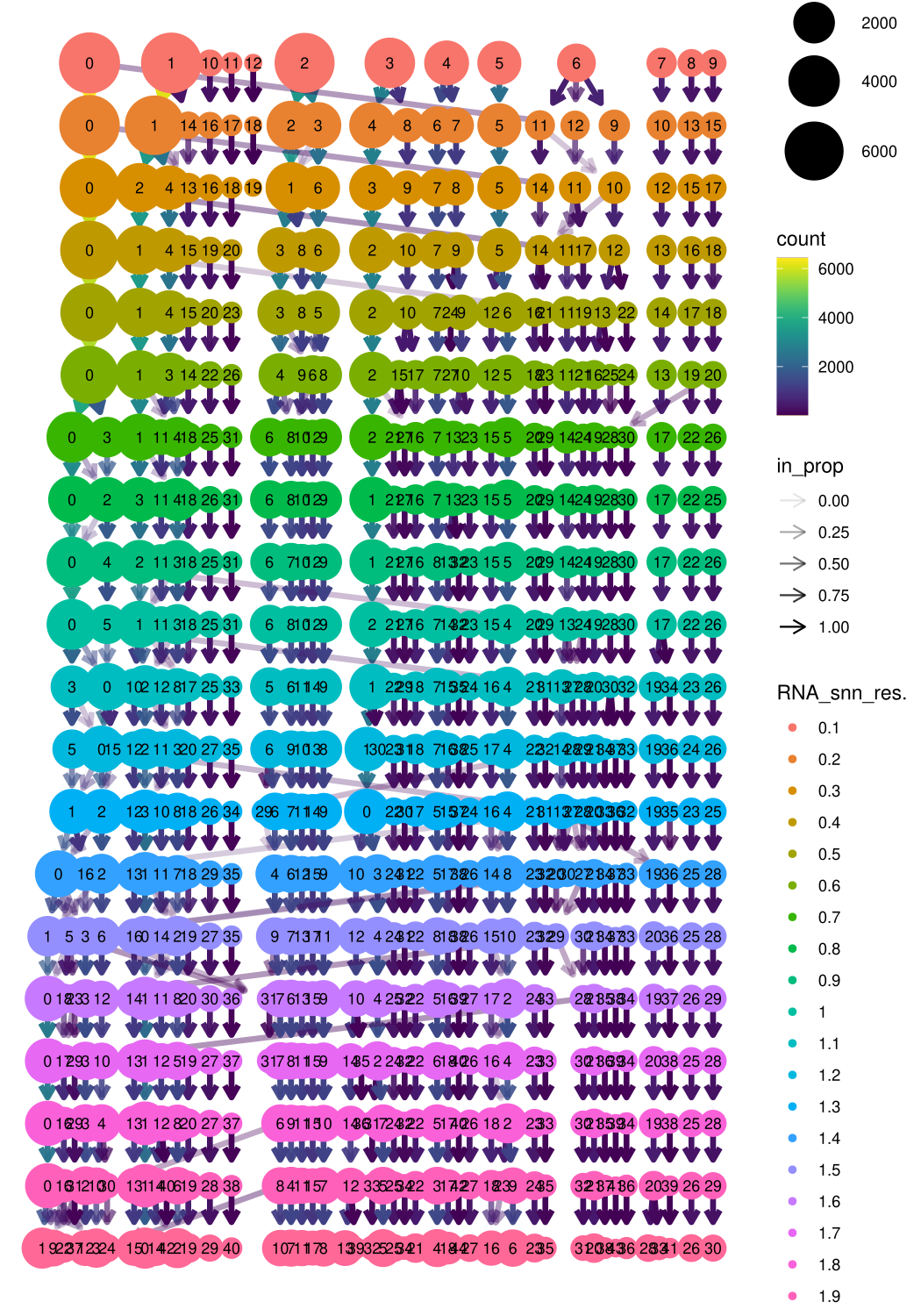
# Here we choose the final resolution for downstream analysis based on clustree
midgut <- FindNeighbors(midgut, dims = 1:15)
midgut <- FindClusters(midgut, resolution = 0.5)
## Modularity Optimizer version 1.3.0 by Ludo Waltman and Nees Jan van Eck
##
## Number of nodes: 31410
## Number of edges: 1084470
##
## Running Louvain algorithm...
## Maximum modularity in 10 random starts: 0.9412
## Number of communities: 25
## Elapsed time: 4 seconds# Look at cluster IDs of the first 10 cells
head(Idents(midgut), 10)## control_AAACCTGAGTGGTAAT-1 control_AAACCTGAGTTGCAGG-1
## 2 17
## control_AAACCTGCAATCGGTT-1 control_AAACCTGCACATTCGA-1
## 2 17
## control_AAACCTGCAGCTCGCA-1 control_AAACCTGCATCGACGC-1
## 2 7
## control_AAACCTGGTGTTCTTT-1 control_AAACCTGTCAGCCTAA-1
## 2 2
## control_AAACCTGTCAGTGTTG-1 control_AAACCTGTCCCTAATT-1
## 7 7
## Levels: 0 1 2 3 4 5 6 7 8 9 10 11 12 13 14 15 16 17 18 19 20 21 22 23 24Run non-linear dimensional reduction (UMAP/tSNE)
Seurat offers several non-linear dimensional reduction techniques, such as tSNE and UMAP, to visualize and explore these datasets. The goal of these algorithms is to learn the underlying manifold of the data in order to place similar cells together in low-dimensional space. Cells within the graph-based clusters determined above should co-localize on these dimension reduction plots. As input to the UMAP and tSNE, we suggest using the same PCs as input to the clustering analysis.
# If you haven't installed UMAP, you can do so via reticulate::py_install(packages = "umap-learn")
midgut <- RunUMAP(midgut, dims = 1:15, reduction = "pca", reduction.name = "umap.unintegrated")

# Here we generate a tSNE embedding.
midgut <- RunTSNE(midgut, dims = 1:15, tsne.method = 'FIt-SNE', reduction = "pca", reduction.name = "tsne.unintegrated")
Then we plot the clusters before integration:
# note that you can set `label = TRUE` or use the LabelClusters function to help label individual clusters
DimPlot(midgut, reduction = "umap.unintegrated")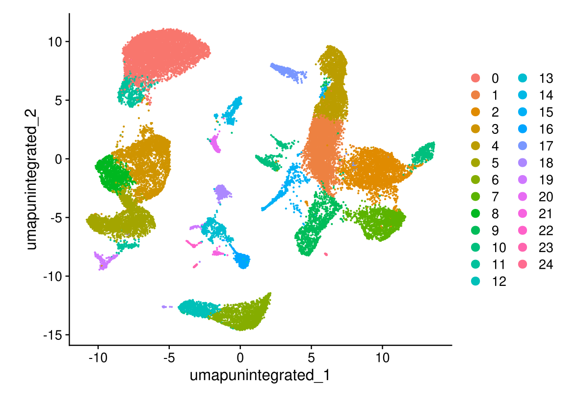
DimPlot(midgut, reduction = "umap.unintegrated", group.by = "technique")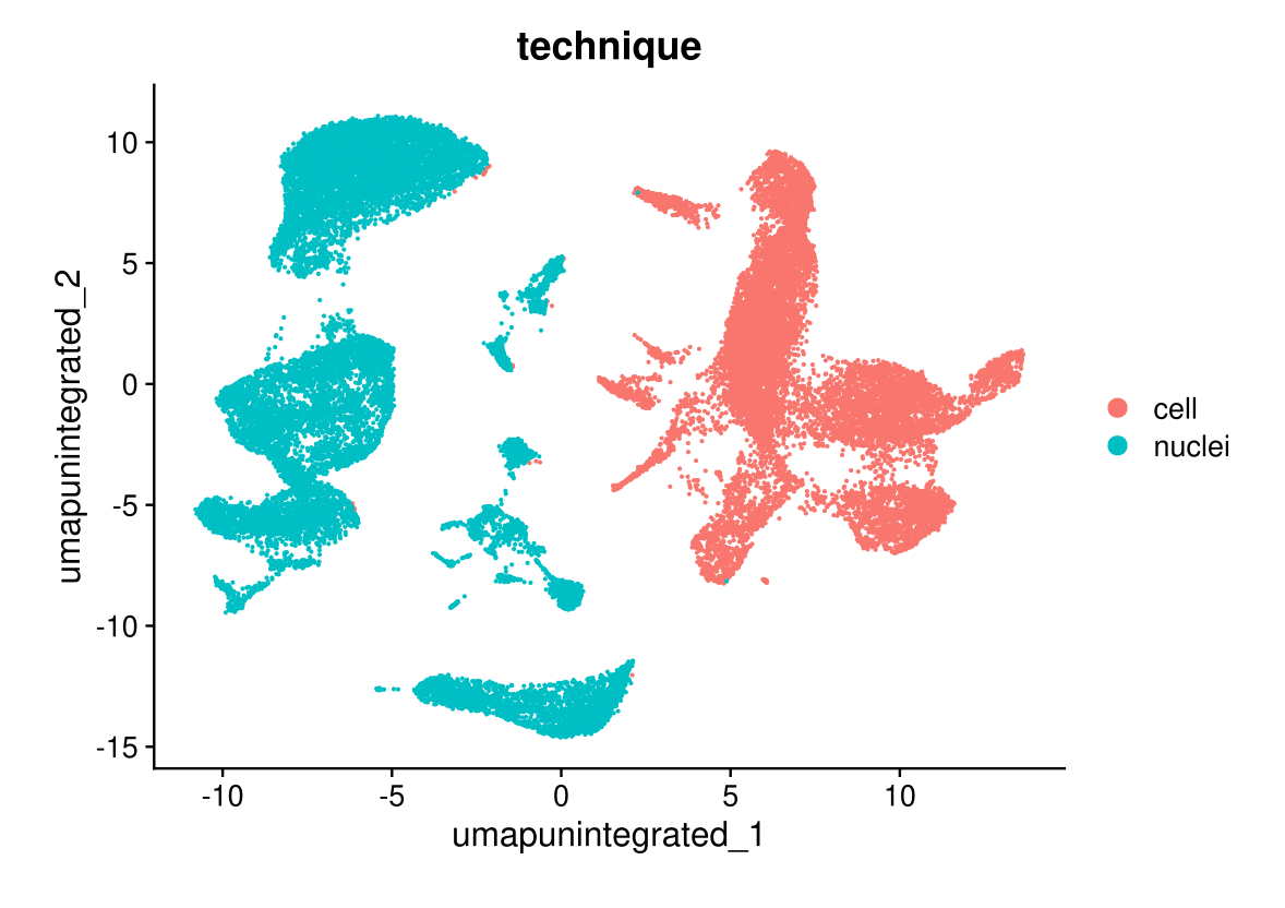
DimPlot(midgut, reduction = "umap.unintegrated", split.by = "technique", label = TRUE, ncol = 2)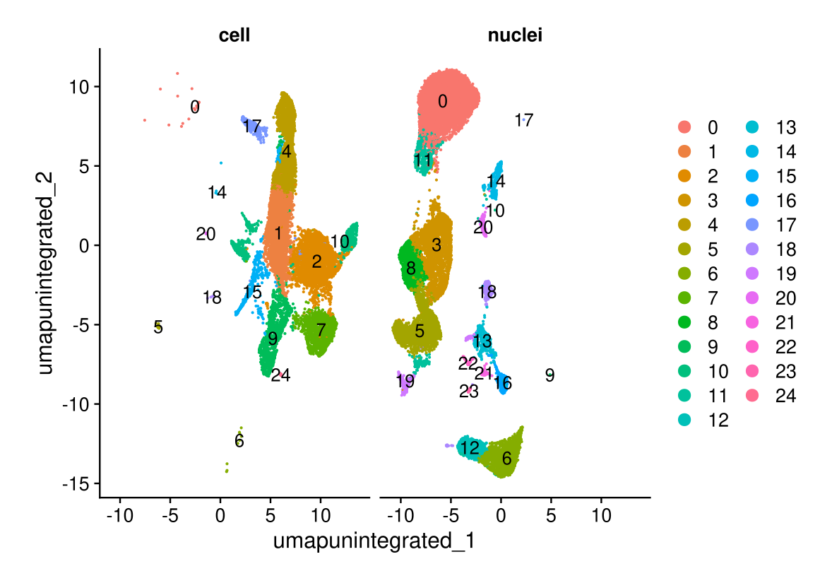
DimPlot(midgut, reduction = "tsne.unintegrated")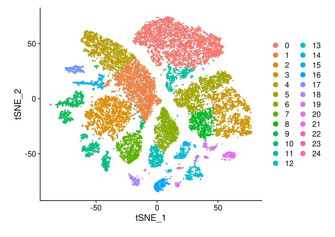
DimPlot(midgut, reduction = "tsne.unintegrated", group.by = "technique")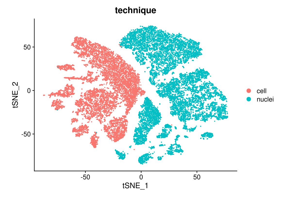
DimPlot(midgut, reduction = "tsne.unintegrated", split.by = "technique", label = TRUE, ncol = 2)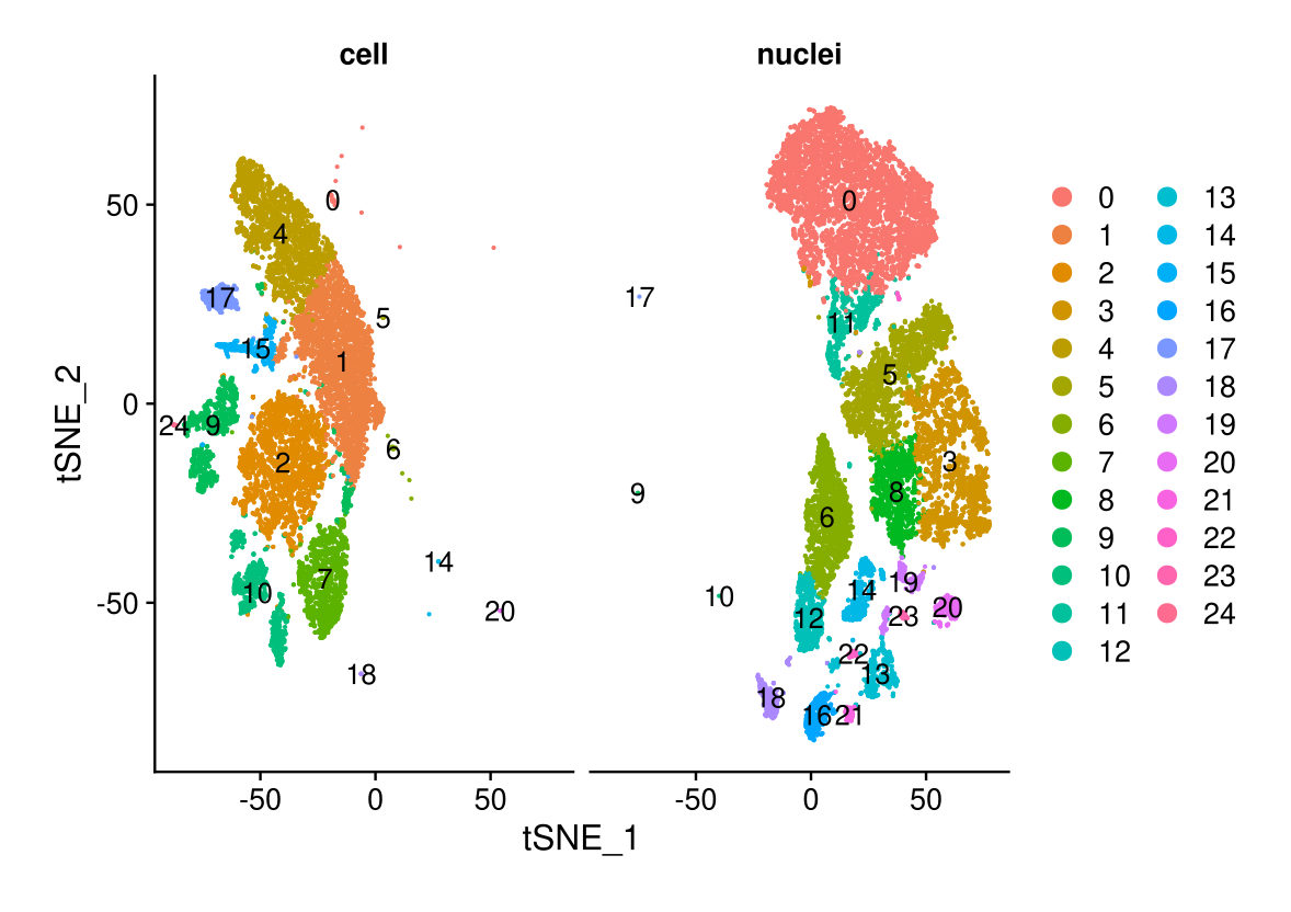
DimPlot(midgut, reduction = "pca")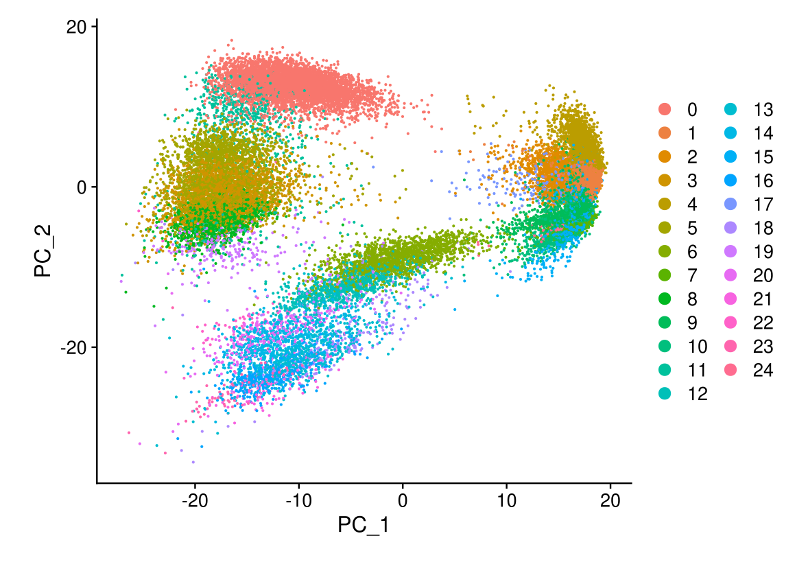
You can save the object at this point so that it can easily be loaded back in without having to rerun the computationally intensive steps performed above, or easily shared with collaborators.
saveRDS(midgut,
        file = "midgut_unintegrated.rds",
        compress = T)
Integrate the data
See https://satijalab.org/seurat/articles/integration_introduction for details
We now aim to integrate data from the two conditions, so that cells from the same cell type/subpopulation will cluster together.
We often refer to this procedure as intergration/alignment. When aligning two genome sequences together, identification of shared/homologous regions can help to interpret differences between the sequences as well. Similarly for scRNA-seq integration, our goal is not to remove biological differences across conditions, but to learn shared cell types/states in an initial step - specifically because that will enable us to compare control stimulated and control profiles for these individual cell types.
The Seurat v5 integration procedure aims to return a single
dimensional reduction that captures the shared sources of variance
across multiple layers, so that cells in a similar biological state will
cluster. The method returns a dimensional reduction
(i.e. integrated.cca) which can be used for visualization
and unsupervised clustering analysis. For evaluating performance, we can
use cell type labels that are pre-loaded in
the seurat_annotations metadata column.
Before the integration, I create different variables for the different models.
midgut.cca <- midgut
midgut.harmony <- midgut
CCA integration
midgut.cca <- IntegrateLayers(object = midgut.cca, method = CCAIntegration, new.reduction = "integrated.cca", verbose = FALSE)

# re-join layers after integration
midgut.cca[["RNA"]] <- JoinLayers(midgut.cca[["RNA"]])

midgut.cca <- FindNeighbors(midgut.cca, reduction = "integrated.cca", dims = 1:15)
midgut.cca <- FindClusters(midgut.cca, resolution = 2)
## Modularity Optimizer version 1.3.0 by Ludo Waltman and Nees Jan van Eck
##
## Number of nodes: 31410
## Number of edges: 1107352
##
## Running Louvain algorithm...
## Maximum modularity in 10 random starts: 0.8489
## Number of communities: 44
## Elapsed time: 5 seconds# cluster assignments at multiple resolutions
resolutions <- c(0.1, 0.2, 0.3, 0.4, 0.5, 0.6, 0.7, 0.8, 0.9, 1.0, 1.1, 1.2, 1.3, 1.4, 1.5) # Example resolutions
for (res in resolutions) {
name <- paste0("RNA_snn_res.", res)
midgut.cca <- FindClusters(midgut.cca, resolution = res, name = name)
}## Modularity Optimizer version 1.3.0 by Ludo Waltman and Nees Jan van Eck
##
## Number of nodes: 31410
## Number of edges: 1107352
##
## Running Louvain algorithm...
## Maximum modularity in 10 random starts: 0.9682
## Number of communities: 11
## Elapsed time: 5 seconds## Modularity Optimizer version 1.3.0 by Ludo Waltman and Nees Jan van Eck
##
## Number of nodes: 31410
## Number of edges: 1107352
##
## Running Louvain algorithm...
## Maximum modularity in 10 random starts: 0.9519
## Number of communities: 14
## Elapsed time: 5 seconds## Modularity Optimizer version 1.3.0 by Ludo Waltman and Nees Jan van Eck
##
## Number of nodes: 31410
## Number of edges: 1107352
##
## Running Louvain algorithm...
## Maximum modularity in 10 random starts: 0.9385
## Number of communities: 15
## Elapsed time: 5 seconds## Modularity Optimizer version 1.3.0 by Ludo Waltman and Nees Jan van Eck
##
## Number of nodes: 31410
## Number of edges: 1107352
##
## Running Louvain algorithm...
## Maximum modularity in 10 random starts: 0.9267
## Number of communities: 19
## Elapsed time: 5 seconds## Modularity Optimizer version 1.3.0 by Ludo Waltman and Nees Jan van Eck
##
## Number of nodes: 31410
## Number of edges: 1107352
##
## Running Louvain algorithm...
## Maximum modularity in 10 random starts: 0.9197
## Number of communities: 22
## Elapsed time: 5 seconds## Modularity Optimizer version 1.3.0 by Ludo Waltman and Nees Jan van Eck
##
## Number of nodes: 31410
## Number of edges: 1107352
##
## Running Louvain algorithm...
## Maximum modularity in 10 random starts: 0.9114
## Number of communities: 23
## Elapsed time: 5 seconds## Modularity Optimizer version 1.3.0 by Ludo Waltman and Nees Jan van Eck
##
## Number of nodes: 31410
## Number of edges: 1107352
##
## Running Louvain algorithm...
## Maximum modularity in 10 random starts: 0.9051
## Number of communities: 25
## Elapsed time: 5 seconds## Modularity Optimizer version 1.3.0 by Ludo Waltman and Nees Jan van Eck
##
## Number of nodes: 31410
## Number of edges: 1107352
##
## Running Louvain algorithm...
## Maximum modularity in 10 random starts: 0.8994
## Number of communities: 29
## Elapsed time: 5 seconds## Modularity Optimizer version 1.3.0 by Ludo Waltman and Nees Jan van Eck
##
## Number of nodes: 31410
## Number of edges: 1107352
##
## Running Louvain algorithm...
## Maximum modularity in 10 random starts: 0.8938
## Number of communities: 28
## Elapsed time: 4 seconds## Modularity Optimizer version 1.3.0 by Ludo Waltman and Nees Jan van Eck
##
## Number of nodes: 31410
## Number of edges: 1107352
##
## Running Louvain algorithm...
## Maximum modularity in 10 random starts: 0.8894
## Number of communities: 31
## Elapsed time: 5 seconds## Modularity Optimizer version 1.3.0 by Ludo Waltman and Nees Jan van Eck
##
## Number of nodes: 31410
## Number of edges: 1107352
##
## Running Louvain algorithm...
## Maximum modularity in 10 random starts: 0.8842
## Number of communities: 34
## Elapsed time: 4 seconds## Modularity Optimizer version 1.3.0 by Ludo Waltman and Nees Jan van Eck
##
## Number of nodes: 31410
## Number of edges: 1107352
##
## Running Louvain algorithm...
## Maximum modularity in 10 random starts: 0.8801
## Number of communities: 34
## Elapsed time: 4 seconds## Modularity Optimizer version 1.3.0 by Ludo Waltman and Nees Jan van Eck
##
## Number of nodes: 31410
## Number of edges: 1107352
##
## Running Louvain algorithm...
## Maximum modularity in 10 random starts: 0.8752
## Number of communities: 34
## Elapsed time: 5 seconds## Modularity Optimizer version 1.3.0 by Ludo Waltman and Nees Jan van Eck
##
## Number of nodes: 31410
## Number of edges: 1107352
##
## Running Louvain algorithm...
## Maximum modularity in 10 random starts: 0.8713
## Number of communities: 39
## Elapsed time: 4 seconds## Modularity Optimizer version 1.3.0 by Ludo Waltman and Nees Jan van Eck
##
## Number of nodes: 31410
## Number of edges: 1107352
##
## Running Louvain algorithm...
## Maximum modularity in 10 random starts: 0.8676
## Number of communities: 37
## Elapsed time: 4 seconds# Refresh metadata after clustering and clustree
Mmeta_data <- midgut.cca@meta.data
clustree(Mmeta_data, prefix = "RNA_snn_res.")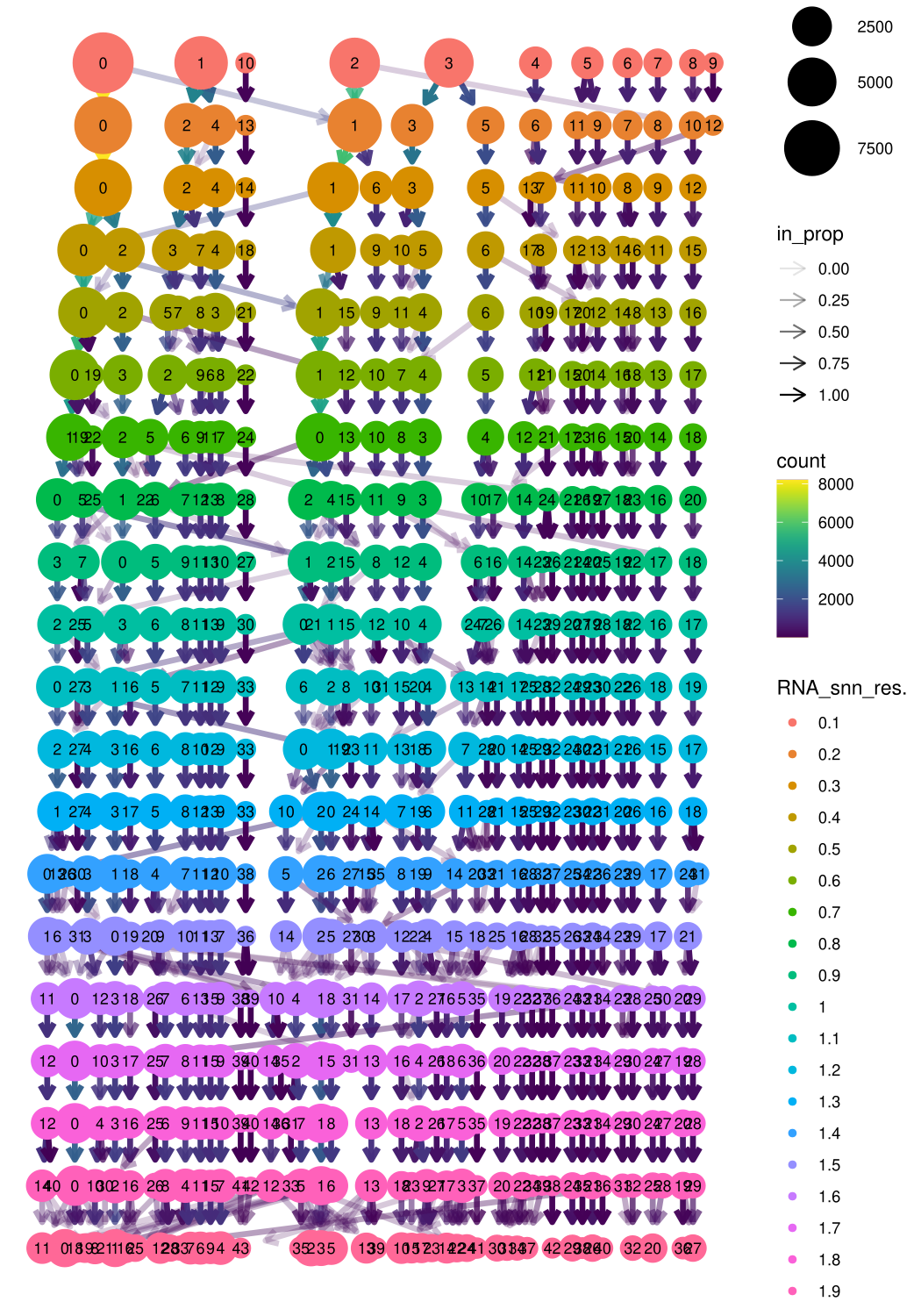
We choose the final clustering
midgut.cca <- FindNeighbors(midgut.cca, reduction = "integrated.cca", dims = 1:15)
midgut.cca <- FindClusters(midgut.cca, resolution = 0.4)
## Modularity Optimizer version 1.3.0 by Ludo Waltman and Nees Jan van Eck
##
## Number of nodes: 31410
## Number of edges: 1107352
##
## Running Louvain algorithm...
## Maximum modularity in 10 random starts: 0.9267
## Number of communities: 19
## Elapsed time: 6 secondsHarmony integration
The same steps as the ones for the CCA are done again here for the Harmony integration
midgut.harmony <- IntegrateLayers(object = midgut.harmony, method = HarmonyIntegration, orig.reduction = "pca", new.reduction = "integrated.harmony", group.by = 'technique', reduction_dims = 1:30, verbose = FALSE)

# re-join layers after integration
midgut.harmony[["RNA"]] <- JoinLayers(midgut.harmony[["RNA"]])

midgut.harmony <- FindNeighbors(midgut.harmony, reduction = "integrated.harmony", dims = 1:30)
midgut.harmony <- FindClusters(midgut.harmony, resolution = 2)
## Modularity Optimizer version 1.3.0 by Ludo Waltman and Nees Jan van Eck
##
## Number of nodes: 31410
## Number of edges: 1210026
##
## Running Louvain algorithm...
## Maximum modularity in 10 random starts: 0.8665
## Number of communities: 47
## Elapsed time: 5 secondslibrary(clustree)
# cluster assignments at multiple resolutions
resolutions <- c(0.1, 0.2, 0.3, 0.4, 0.5, 0.6, 0.7, 0.8, 0.9, 1.0, 1.1, 1.2, 1.3, 1.4, 1.5) # Example resolutions
for (res in resolutions) {
name <- paste0("RNA_snn_res.", res)
midgut.harmony <- FindClusters(midgut.harmony, resolution = res, name = name)
}## Modularity Optimizer version 1.3.0 by Ludo Waltman and Nees Jan van Eck
##
## Number of nodes: 31410
## Number of edges: 1210026
##
## Running Louvain algorithm...
## Maximum modularity in 10 random starts: 0.9792
## Number of communities: 15
## Elapsed time: 5 seconds## Modularity Optimizer version 1.3.0 by Ludo Waltman and Nees Jan van Eck
##
## Number of nodes: 31410
## Number of edges: 1210026
##
## Running Louvain algorithm...
## Maximum modularity in 10 random starts: 0.9639
## Number of communities: 18
## Elapsed time: 5 seconds## Modularity Optimizer version 1.3.0 by Ludo Waltman and Nees Jan van Eck
##
## Number of nodes: 31410
## Number of edges: 1210026
##
## Running Louvain algorithm...
## Maximum modularity in 10 random starts: 0.9527
## Number of communities: 22
## Elapsed time: 5 seconds## Modularity Optimizer version 1.3.0 by Ludo Waltman and Nees Jan van Eck
##
## Number of nodes: 31410
## Number of edges: 1210026
##
## Running Louvain algorithm...
## Maximum modularity in 10 random starts: 0.9432
## Number of communities: 26
## Elapsed time: 6 seconds## Modularity Optimizer version 1.3.0 by Ludo Waltman and Nees Jan van Eck
##
## Number of nodes: 31410
## Number of edges: 1210026
##
## Running Louvain algorithm...
## Maximum modularity in 10 random starts: 0.9347
## Number of communities: 27
## Elapsed time: 5 seconds## Modularity Optimizer version 1.3.0 by Ludo Waltman and Nees Jan van Eck
##
## Number of nodes: 31410
## Number of edges: 1210026
##
## Running Louvain algorithm...
## Maximum modularity in 10 random starts: 0.9274
## Number of communities: 31
## Elapsed time: 6 seconds## Modularity Optimizer version 1.3.0 by Ludo Waltman and Nees Jan van Eck
##
## Number of nodes: 31410
## Number of edges: 1210026
##
## Running Louvain algorithm...
## Maximum modularity in 10 random starts: 0.9203
## Number of communities: 31
## Elapsed time: 5 seconds## Modularity Optimizer version 1.3.0 by Ludo Waltman and Nees Jan van Eck
##
## Number of nodes: 31410
## Number of edges: 1210026
##
## Running Louvain algorithm...
## Maximum modularity in 10 random starts: 0.9142
## Number of communities: 33
## Elapsed time: 5 seconds## Modularity Optimizer version 1.3.0 by Ludo Waltman and Nees Jan van Eck
##
## Number of nodes: 31410
## Number of edges: 1210026
##
## Running Louvain algorithm...
## Maximum modularity in 10 random starts: 0.9081
## Number of communities: 36
## Elapsed time: 5 seconds## Modularity Optimizer version 1.3.0 by Ludo Waltman and Nees Jan van Eck
##
## Number of nodes: 31410
## Number of edges: 1210026
##
## Running Louvain algorithm...
## Maximum modularity in 10 random starts: 0.9035
## Number of communities: 36
## Elapsed time: 6 seconds## Modularity Optimizer version 1.3.0 by Ludo Waltman and Nees Jan van Eck
##
## Number of nodes: 31410
## Number of edges: 1210026
##
## Running Louvain algorithm...
## Maximum modularity in 10 random starts: 0.8988
## Number of communities: 37
## Elapsed time: 6 seconds## Modularity Optimizer version 1.3.0 by Ludo Waltman and Nees Jan van Eck
##
## Number of nodes: 31410
## Number of edges: 1210026
##
## Running Louvain algorithm...
## Maximum modularity in 10 random starts: 0.8940
## Number of communities: 40
## Elapsed time: 4 seconds## Modularity Optimizer version 1.3.0 by Ludo Waltman and Nees Jan van Eck
##
## Number of nodes: 31410
## Number of edges: 1210026
##
## Running Louvain algorithm...
## Maximum modularity in 10 random starts: 0.8898
## Number of communities: 39
## Elapsed time: 4 seconds## Modularity Optimizer version 1.3.0 by Ludo Waltman and Nees Jan van Eck
##
## Number of nodes: 31410
## Number of edges: 1210026
##
## Running Louvain algorithm...
## Maximum modularity in 10 random starts: 0.8861
## Number of communities: 42
## Elapsed time: 4 seconds## Modularity Optimizer version 1.3.0 by Ludo Waltman and Nees Jan van Eck
##
## Number of nodes: 31410
## Number of edges: 1210026
##
## Running Louvain algorithm...
## Maximum modularity in 10 random starts: 0.8829
## Number of communities: 42
## Elapsed time: 5 seconds# Refresh metadata after clustering and clustree
Mmeta_data <- midgut.harmony@meta.data
clustree(Mmeta_data, prefix = "RNA_snn_res.")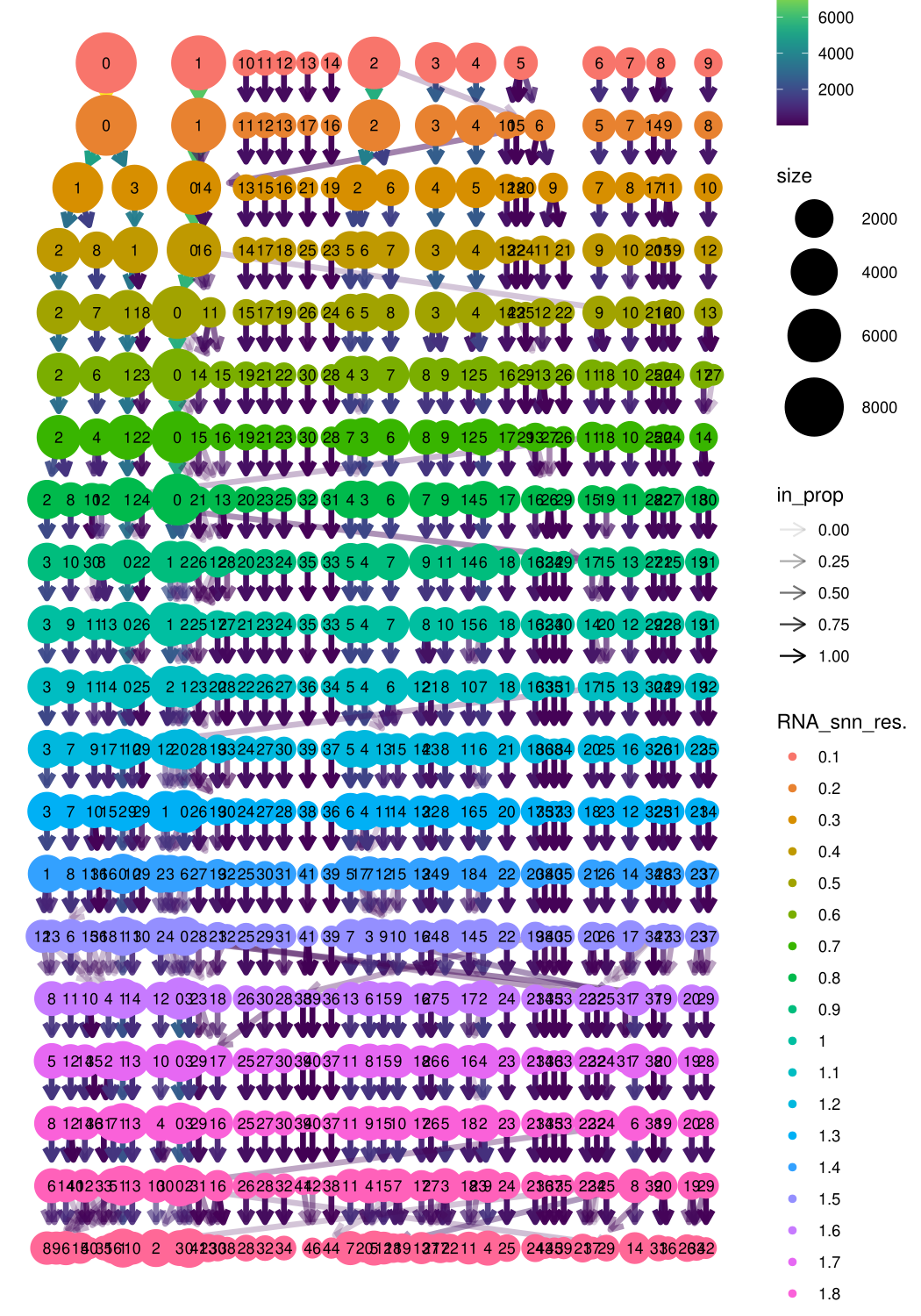
midgut.harmony <- FindNeighbors(midgut.harmony, reduction = "integrated.harmony", dims = 1:30)
midgut.harmony <- FindClusters(midgut.harmony, resolution = 0.4)
## Modularity Optimizer version 1.3.0 by Ludo Waltman and Nees Jan van Eck
##
## Number of nodes: 31410
## Number of edges: 1210026
##
## Running Louvain algorithm...
## Maximum modularity in 10 random starts: 0.9432
## Number of communities: 26
## Elapsed time: 6 secondsVisualization after integration
First we generate UMAP and tSNE
# Here we generate a UMAP embedding
midgut.cca <- RunUMAP(midgut.cca, dims = 1:15, reduction="integrated.cca", reduction.name = "umap.integrated.cca")
midgut.harmony <- RunUMAP(midgut.harmony, dims = 1:15, reduction="integrated.harmony", reduction.name = "umap.integrated.harmony")

# Here we generate a tSNE embedding
midgut.cca <- RunTSNE(midgut.cca, dims = 1:15, tsne.method = 'FIt-SNE', reduction="integrated.cca", reduction.name = "tsne.integrated.cca")
midgut.harmony <- RunTSNE(midgut.harmony, dims = 1:15, tsne.method = 'FIt-SNE', reduction="integrated.harmony", reduction.name = "tsne.integrated.harmony")
And we visualize the results of the different integration models
DimPlot(midgut.cca, reduction = "umap.integrated.cca")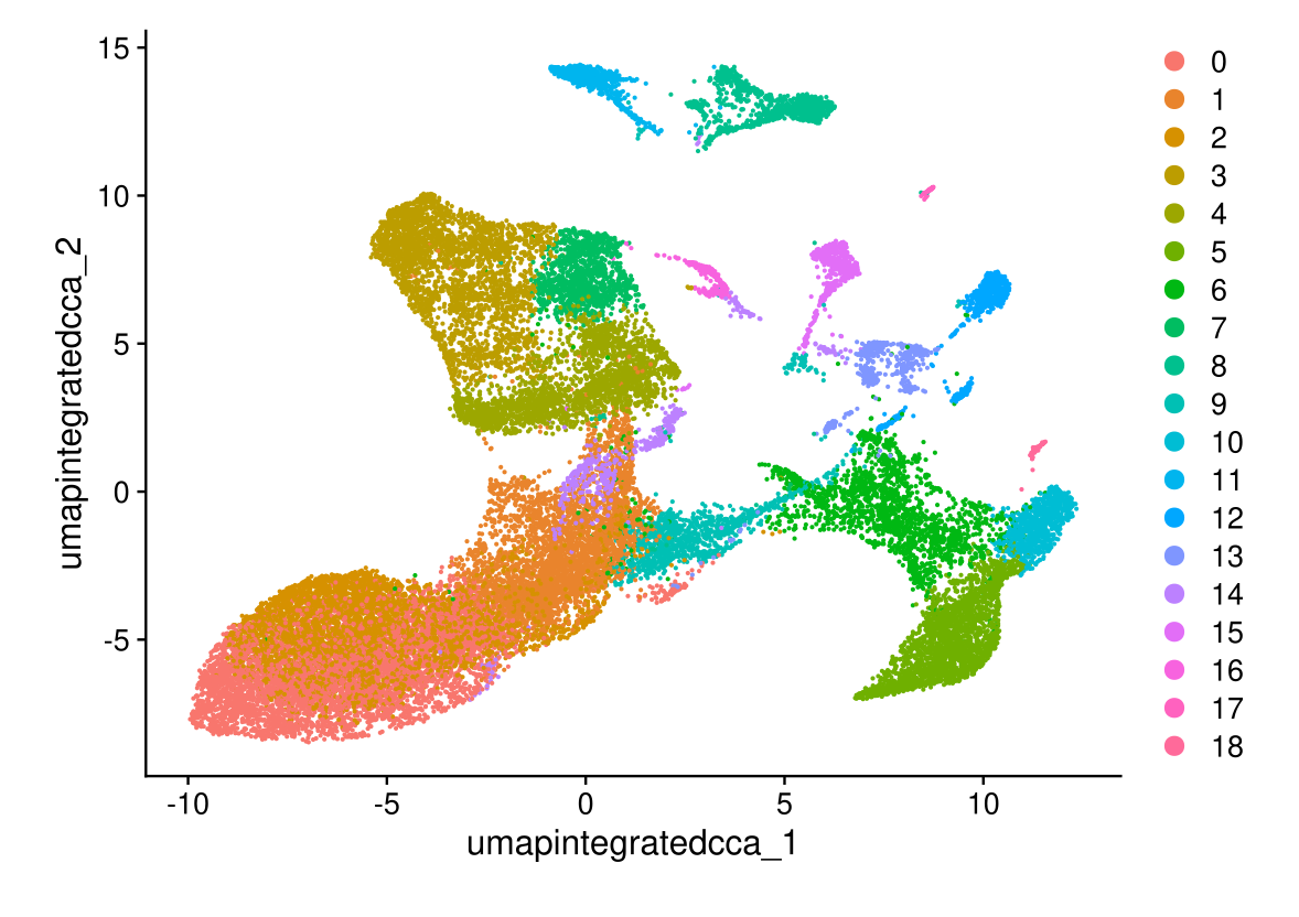
DimPlot(midgut.cca, reduction = "umap.integrated.cca", group.by = "technique", alpha = 0.4)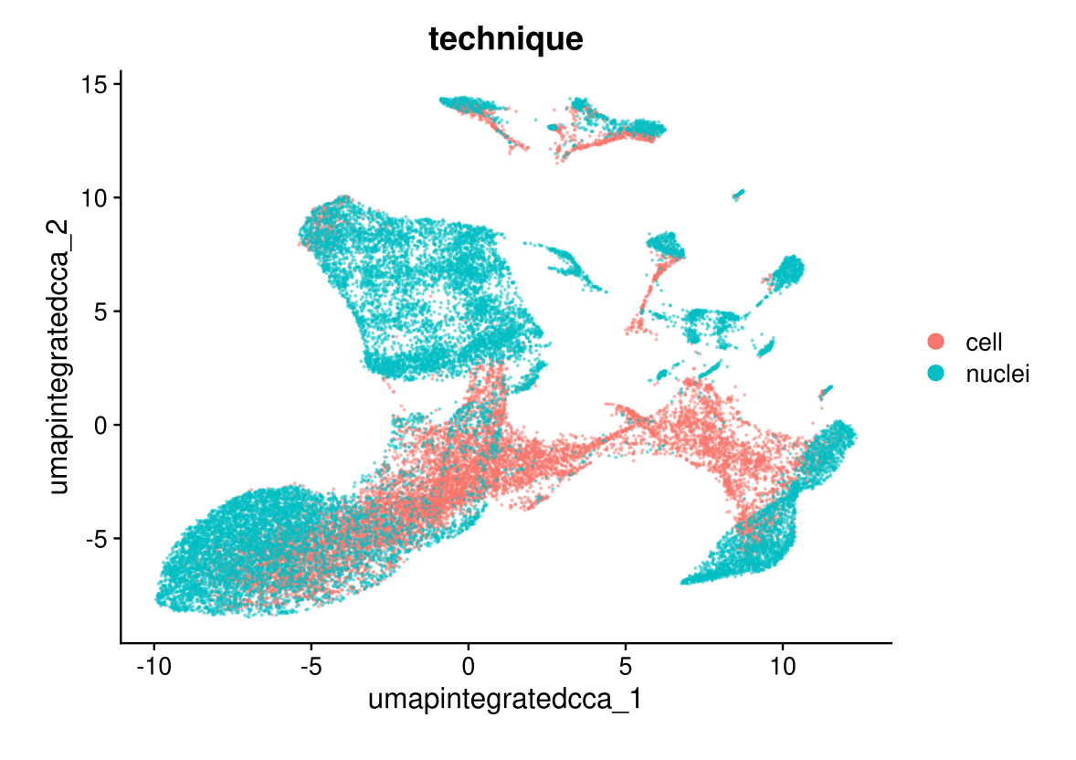
DimPlot(midgut.cca, reduction = "umap.integrated.cca", split.by = "technique", label = TRUE, ncol = 2)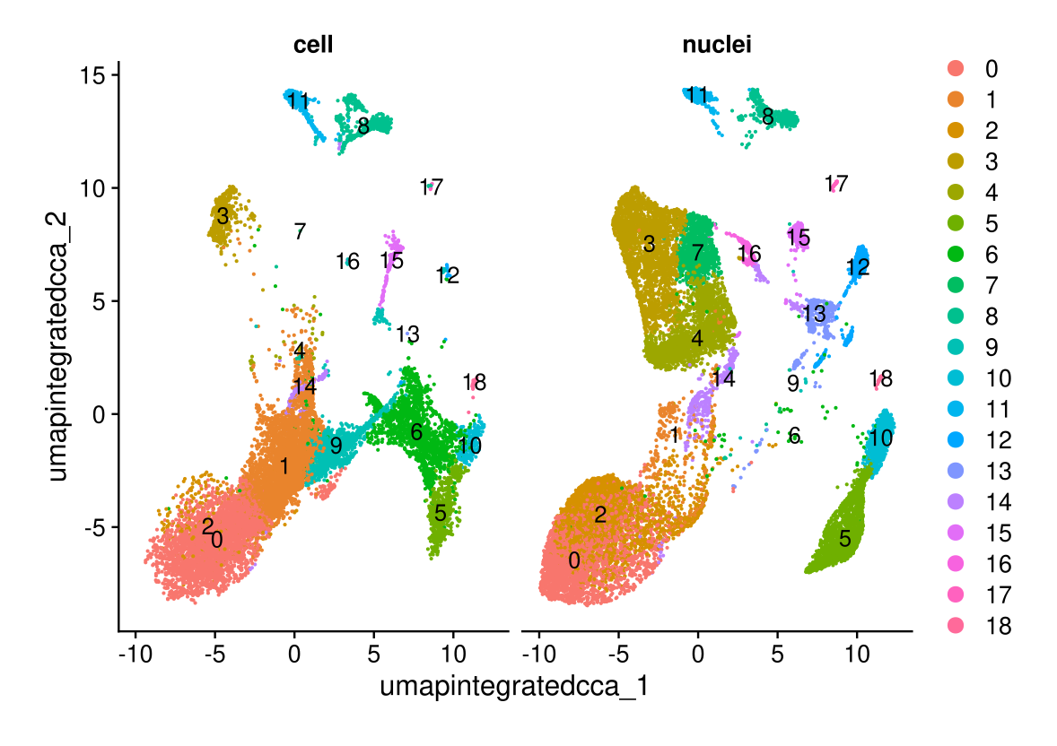
DimPlot(midgut.cca, reduction = "tsne.integrated.cca")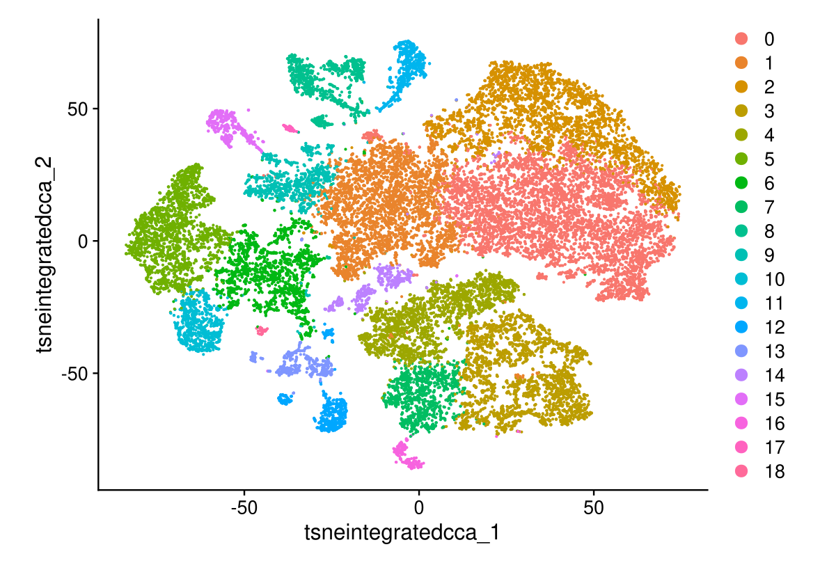
DimPlot(midgut.cca, reduction = "tsne.integrated.cca", group.by = "technique", alpha = 0.4)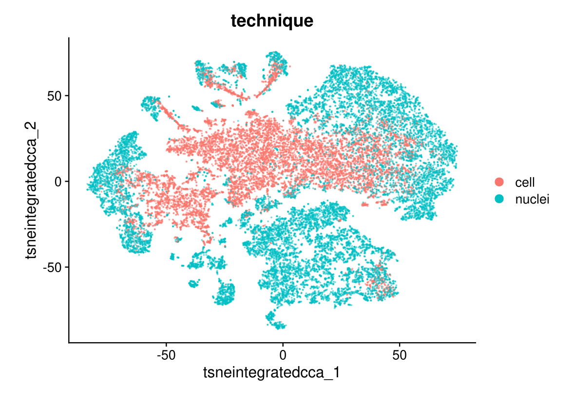
DimPlot(midgut.cca, reduction = "tsne.integrated.cca", split.by = "technique")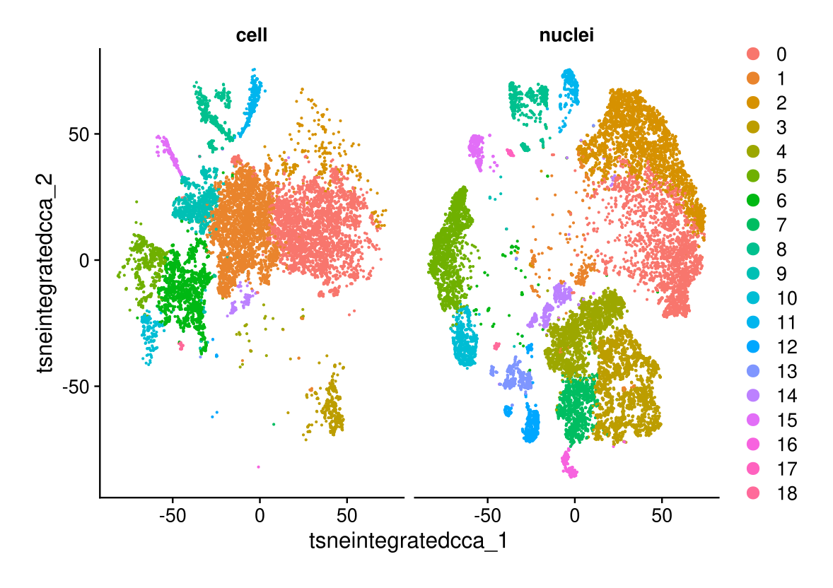
DimPlot(midgut.harmony, reduction = "umap.integrated.harmony")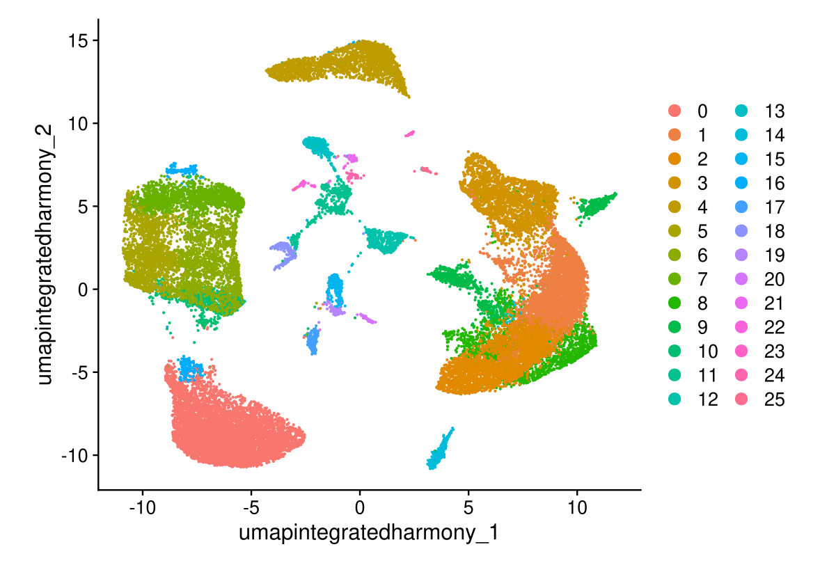
DimPlot(midgut.harmony, reduction = "umap.integrated.harmony", group.by = "technique", alpha = 0.4)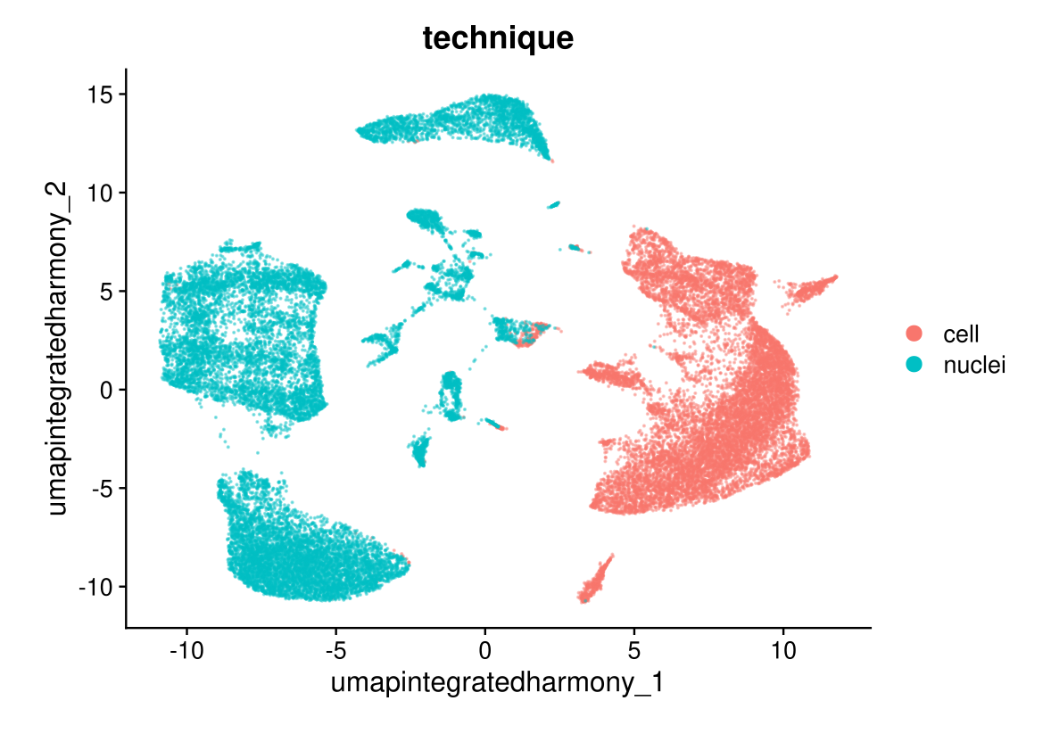
DimPlot(midgut.harmony, reduction = "umap.integrated.harmony", split.by = "technique", label = TRUE, ncol = 2)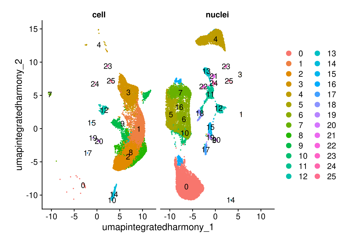
DimPlot(midgut.harmony, reduction = "tsne.integrated.harmony")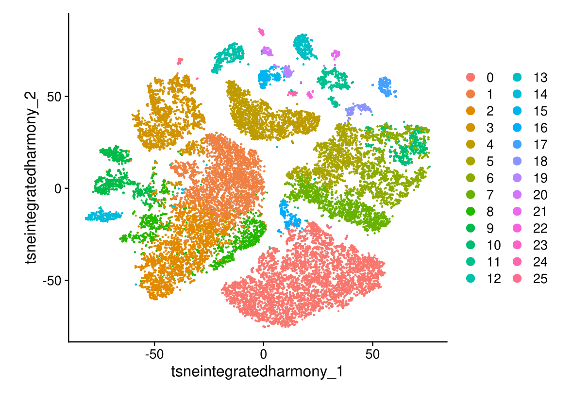
DimPlot(midgut.harmony, reduction = "tsne.integrated.harmony", group.by = "technique", alpha = 0.4)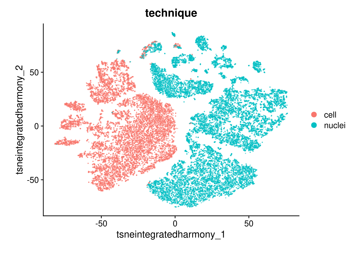
DimPlot(midgut.harmony, reduction = "tsne.integrated.harmony", split.by = "technique")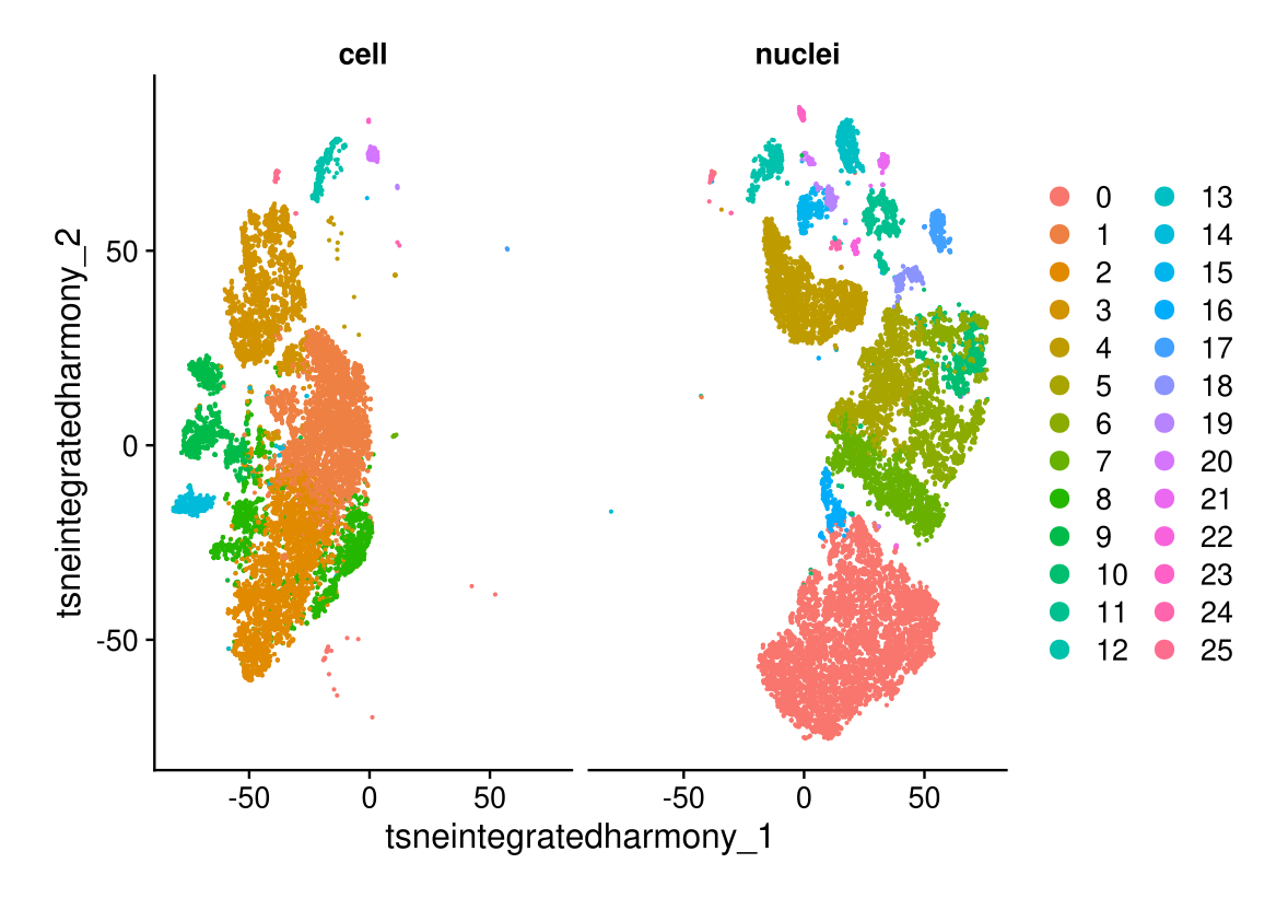
Comparison between techniques
Here we generate a table with all the numbers of cells and nuclei by cluster and their proportionsa and we export the results in an excel file.
# Creates a data frame that counts the number of cells for each combination of cluster identity and technique in midgut.cc
df <- as.data.frame(table(
  cluster = Idents(midgut.cca),
  technique = midgut.cca$technique
))

# Create a summary table with df data
summary_table <- df |>
  tidyr::pivot_wider(names_from = technique, values_from = Freq, values_fill = 0) |>
  mutate(
    total = nuclei + cell,
    `% nuclei` = round(100 * nuclei / total, 1),
    `% cell` = round(100 * cell / total, 1)
  ) |>
  select(cluster, total, nuclei, cell, `% nuclei`, `% cell`) |>
  arrange(as.numeric(as.character(cluster)))

# Excel export
write_xlsx(summary_table, "cluster_summary.xlsx")
And we generate a diagram that plot the proportion of each technique that is contributing to a cluster.
# Plot the propotion of each technique contributing to a cluster
df <- as.data.frame(table(cluster = Idents(midgut.cca), technique = midgut.cca$technique))

ggplot(df, aes(y = factor(cluster), x = Freq, fill = technique)) +
  geom_bar(stat = "identity", position = "fill") +
  xlab("Proportion") +
  ylab("Cluster") +
  theme_minimal()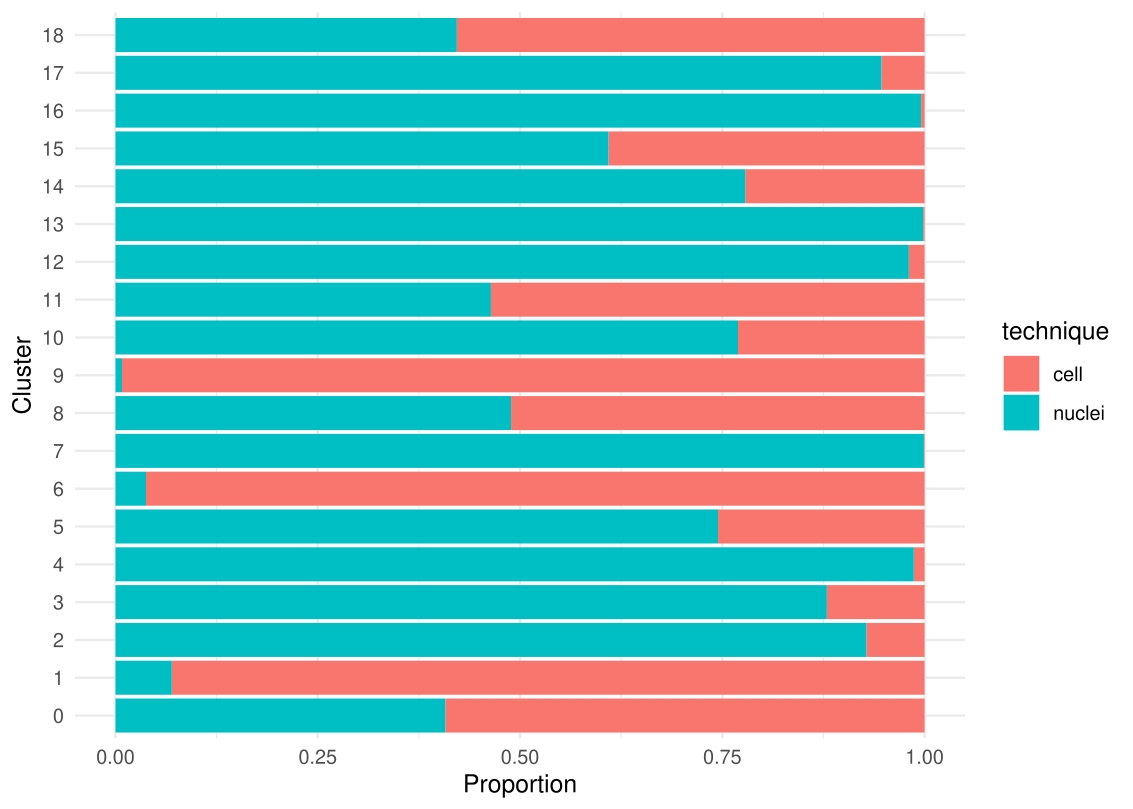
Finding differentially expressed features (cluster biomarkers)
Seurat can help you find markers that define clusters via
differential expression. By default, it identifies positive and negative
markers of a single cluster (specified in ident.1),
compared to all other cells. FindAllMarkers() automates
this process for all clusters, but you can also test groups of clusters
vs. each other, or against all cells.
The min.pct argument requires a feature to be detected
at a minimum percentage in either of the two groups of cells, and the
thresh.test argument requires a feature to be differentially expressed
(on average) by some amount between the two groups. You can set both of
these to 0, but with a dramatic increase in time - since this will test
a large number of features that are unlikely to be highly
discriminatory. As another option to speed up these computations,
max.cells.per.ident can be set. This will downsample each
identity class to have no more cells than whatever this is set to. While
there is generally going to be a loss in power, the speed increases can
be significant and the most highly differentially expressed features
will likely still rise to the top.
# find markers for every cluster compared to all remaining cells, report only the positive ones
midgut.cca.markers <- FindAllMarkers(midgut.cca, only.pos = TRUE, min.pct = 0.25, logfc.threshold = 0.25)

# Select top 10 marker genes by cluster
top_n <- 10

top_markers <- midgut.cca.markers |>
  group_by(cluster) |>
  top_n(n = top_n, wt = avg_log2FC) |>
  arrange(cluster, desc(avg_log2FC)) |>
  mutate(rank = row_number())

# Convert the table: 1 cluster = 1 row
marker_table <- top_markers |>
  select(cluster, rank, gene) |>
  pivot_wider(
    names_from = rank,
    values_from = gene,
    names_prefix = "marker_"
  ) |>
  arrange(as.numeric(as.character(cluster)))

# Excel export
write_xlsx(marker_table, "cluster_marker_table.xlsx")
Finaly, with all these information, we compare the marker genes with the gene expression in: - nuclei mosquito atlas, [https://cells.ucsc.edu/?ds=mosquito+t012] - cell mosquito atlas (mock), [https://aedes-cell-atlas.pasteur.cloud/midgut/]
And we save all the important data and information to avoid running again the whole pipeline.
saveRDS(midgut,
        file = "midgut_integrated.rds",
        compress = T)
save.image(file = "my_work_space.RData", compress = T)Session Info
sessionInfo()## R version 4.5.0 (2025-04-11)
## Platform: x86_64-pc-linux-gnu
## Running under: Ubuntu 20.04.6 LTS
##
## Matrix products: default
## BLAS: /usr/local/lib/R/lib/libRblas.so
## LAPACK: /usr/local/lib/R/lib/libRlapack.so; LAPACK version 3.12.1
##
## locale:
## [1] LC_CTYPE=en_US.UTF-8 LC_NUMERIC=C
## [3] LC_TIME=en_US.UTF-8 LC_COLLATE=en_US.UTF-8
## [5] LC_MONETARY=en_US.UTF-8 LC_MESSAGES=en_US.UTF-8
## [7] LC_PAPER=en_US.UTF-8 LC_NAME=C
## [9] LC_ADDRESS=C LC_TELEPHONE=C
## [11] LC_MEASUREMENT=en_US.UTF-8 LC_IDENTIFICATION=C
##
## time zone: Etc/UTC
## tzcode source: system (glibc)
##
## attached base packages:
## [1] stats graphics grDevices utils datasets methods base
##
## other attached packages:
## [1] future_1.49.0 writexl_1.5.4 tidyr_1.3.1 openxlsx_4.2.8
## [5] anndata_0.7.5.6 scCustomize_3.0.1 sceasy_0.0.7 reticulate_1.42.0
## [9] clustree_0.5.1 ggraph_2.2.1 ggplot2_3.5.2 patchwork_1.3.0
## [13] Seurat_5.3.0 dplyr_1.1.4 SeuratObject_5.1.0 sp_2.2-0
## [17] Matrix_1.7-3
##
## loaded via a namespace (and not attached):
## [1] RColorBrewer_1.1-3 shape_1.4.6.1 rstudioapi_0.17.1
## [4] jsonlite_2.0.0 magrittr_2.0.3 spatstat.utils_3.1-3
## [7] ggbeeswarm_0.7.2 farver_2.1.2 rmarkdown_2.29
## [10] GlobalOptions_0.1.2 vctrs_0.6.5 ROCR_1.0-11
## [13] memoise_2.0.1 spatstat.explore_3.4-2 paletteer_1.6.0
## [16] janitor_2.2.1 forcats_1.0.0 htmltools_0.5.8.1
## [19] sass_0.4.10 sctransform_0.4.2 parallelly_1.44.0
## [22] KernSmooth_2.23-26 bslib_0.9.0 htmlwidgets_1.6.4
## [25] ica_1.0-3 plyr_1.8.9 lubridate_1.9.4
## [28] plotly_4.10.4 zoo_1.8-14 cachem_1.1.0
## [31] igraph_2.1.4 mime_0.13 lifecycle_1.0.4
## [34] pkgconfig_2.0.3 R6_2.6.1 fastmap_1.2.0
## [37] snakecase_0.11.1 fitdistrplus_1.2-2 shiny_1.10.0
## [40] digest_0.6.37 colorspace_2.1-1 rematch2_2.1.2
## [43] tensor_1.5 RSpectra_0.16-2 irlba_2.3.5.1
## [46] labeling_0.4.3 progressr_0.15.1 timechange_0.3.0
## [49] spatstat.sparse_3.1-0 httr_1.4.7 polyclip_1.10-7
## [52] abind_1.4-8 compiler_4.5.0 withr_3.0.2
## [55] backports_1.5.0 viridis_0.6.5 fastDummies_1.7.5
## [58] ggforce_0.4.2 MASS_7.3-65 tools_4.5.0
## [61] vipor_0.4.7 lmtest_0.9-40 beeswarm_0.4.0
## [64] zip_2.3.2 httpuv_1.6.16 future.apply_1.11.3
## [67] goftest_1.2-3 glue_1.8.0 nlme_3.1-168
## [70] promises_1.3.2 grid_4.5.0 checkmate_2.3.2
## [73] Rtsne_0.17 cluster_2.1.8.1 reshape2_1.4.4
## [76] generics_0.1.4 gtable_0.3.6 spatstat.data_3.1-6
## [79] data.table_1.17.2 tidygraph_1.3.1 spatstat.geom_3.3-6
## [82] RcppAnnoy_0.0.22 ggrepel_0.9.6 RANN_2.6.2
## [85] pillar_1.10.2 stringr_1.5.1 ggprism_1.0.5
## [88] spam_2.11-1 RcppHNSW_0.6.0 later_1.4.2
## [91] circlize_0.4.16 splines_4.5.0 tweenr_2.0.3
## [94] lattice_0.22-6 survival_3.8-3 deldir_2.0-4
## [97] tidyselect_1.2.1 miniUI_0.1.2 pbapply_1.7-2
## [100] knitr_1.50 gridExtra_2.3 scattermore_1.2
## [103] RhpcBLASctl_0.23-42 xfun_0.52 graphlayouts_1.2.2
## [106] matrixStats_1.5.0 stringi_1.8.7 lazyeval_0.2.2
## [109] yaml_2.3.10 evaluate_1.0.3 codetools_0.2-20
## [112] tibble_3.2.1 cli_3.6.5 uwot_0.2.3
## [115] xtable_1.8-4 jquerylib_0.1.4 harmony_1.2.3
## [118] Rcpp_1.0.14 globals_0.18.0 spatstat.random_3.3-3
## [121] png_0.1-8 ggrastr_1.0.2 spatstat.univar_3.1-3
## [124] parallel_4.5.0 assertthat_0.2.1 dotCall64_1.2
## [127] listenv_0.9.1 viridisLite_0.4.2 scales_1.4.0
## [130] ggridges_0.5.6 purrr_1.0.4 rlang_1.1.6
## [133] cowplot_1.1.3